Table of Contents
The article is organized as an empirical analysis followed by a detailed technical appendix.
Executive Summary
What Price Discovery Means—and Why These Four Markets
Volume Is Not Information
How the Study Measures Price Discovery
What Previous Studies Found—and Why They Disagree
Data Construction, Normalization, and Claim Limits
The Durable-Price Ranking Does Not Survive the Estimator
Which Market Moves First Changes Around the Clock
Fast Does Not Always Mean Adopted
Information-Arrival Regimes
9.1 Consumer Prices and Federal Reserve Decisions
9.2 Allocator Flows
9.3 CME Weekend Availability
Stablecoins Are Numeraires, Funding Variables, and Tail Risks—Not a Fifth Venue
A Practical Regime Map
What the Shifting First-Response Market Means
For Traders
For Execution Desks
For Allocators
For Risk Managers
For Regulators
Limitations
Conclusion
Technical Appendix
A. Data Sources and Quality
B. Method Provenance, Formulas, and Symbol Guide
C. Category Construction
D. Daily Pairwise Common-Price Model
E. Temporal-Precedence Model
F. Persistence Analysis
G. Event Modules
G.1 Scheduled Macro Events
G.2 Allocator-Flow Regimes
G.3 Leverage-Stress Proxies
G.4 CME Weekend Schedule Expansion
H. Stablecoin and Category Robustness
I. Continuous Quote and Execution-Quality Results
J. Sampled Depth, Trade Size, and Direct Liquidations
K. USDT, USDC, and Stablecoin Supply
References and Evidence Notes
The market that moves first changes across hours and events; no single market consistently owns the durable price. Quote, depth, liquidation and stablecoin evidence show that market structure - not turnover alone - shapes those shifts.

Executive summary
Price discovery is not the same as trading activity. It asks how valuation-relevant information enters linked Bitcoin prices: which market moves first, which price the others adjust toward, which category contributes to the shared non-mean-reverting price, and how much of an initial move survives. The study compares spot, offshore perpetuals, CME futures and U.S. spot Bitcoin ETFs because each provides a directly tradable Bitcoin-linked price, economically material activity, an observable arbitrage or hedging link, and sufficiently consistent minute-level data. Stablecoins remain funding and denomination variables rather than a fifth Bitcoin price venue.
Perpetuals generated 68.0% of selected-venue notional turnover in the common U.S. window, versus 14.5% for ETFs, 9.3% for CME and 8.3% for spot. Yet each category received roughly one quarter of the three durable-price attribution scores. Perpetuals traded the most, but their turnover share was 2.78 times their noise-adjusted information-leadership score. Volume is not information.
The durable-price ranking remains shared and estimator-sensitive. Hasbrouck Information Share and Component Share tilt slightly toward spot and perpetuals; Information Leadership Share tilts slightly toward CME and ETFs. The scores are close, confidence intervals overlap, and the ETF edge disappears under a five-fund return composite. No permanent four-market winner survives the estimator and representation checks.
The trade-price 7 x 24 map identifies 73 statistically distinguishable hour cells: 42 for perpetuals and 31 for CME; 95 remain uncertain. A trade price records an executed transaction, while a quote midpoint is the price halfway between the best bid and ask. The complementary quote-midpoint analysis finds that perpetuals lead spot by 0.0061 and the five-fund ETF quote composite leads spot by 0.0064. The ETF-perpetual difference is statistically indistinguishable from zero because its interval runs from -0.0011 to 0.0028.
A daily regression asks what predicts the perpetual-over-spot quote-timing score. A turnover-only benchmark uses relative turnover because market commentary often treats heavy trading as evidence that a venue should react first. A second model uses relative top-of-book quote size, imbalance, volatility, quote inactivity and spread. The turnover benchmark explains 9.4% of in-sample variation and performs worse than a constant-mean forecast out of sample. The market-structure model explains 48.9% in sample and reduces held-out squared prediction error by 32.1% relative to the constant-mean benchmark. That is economically meaningful for a noisy daily timing measure, but it still leaves most day-to-day variation unexplained.
Direct liquidation records permit a matched-event stress comparison. The study selects large liquidation minutes and pairs each with a same-day non-liquidation price shock of similar initial size. Across 67 pairs, liquidation-originating moves have median persistence of 0.46 at 30 minutes and 0.00 at two hours, versus 1.31 and 1.29 for the controls. Repeated resampling puts the two-hour continuation difference between -49.7 and -0.0 basis points, barely below zero, while a rank-based test gives p=0.099. The sign and size point toward reversal, but the evidence is not conclusive because the statistical tests do not agree at the conventional 5% threshold.
USDC usually trades closer to one dollar than USDT, but it experienced a much larger tail event in March 2023 after Circle disclosed that $3.3 billion of its reserves were held at the failed Silicon Valley Bank; the peg recovered after U.S. authorities protected the bank’s depositors [25][26]. A one-minute peg-return correction is simply the minute change in the stablecoin’s dollar price that must be added when a BTC/stablecoin return is expressed in dollars. Its standard deviation is 0.67 basis points for USDT and 0.98 for USDC, so the usual minute-by-minute effect is small even though depegs can be large. Using prior-day supply changes to predict next-day spot-perpetual timing adds no robust signal: the joint test gives p=0.758, and held-out forecasts worsen when the supply variables are included.
Scheduled and allocator events remain regime-dependent. CME has the clearest trade-price first-response result around CPI, while FOMC timing is mixed. Continuous quote data show that crypto spreads remain very tight around those announcements; ETF spreads are structurally wider during the regular session. On large ETF inflow days, ETF quotes lead spot and remain competitive with perpetuals, but large outflow days shift the timing balance toward perpetuals. High ETF volume with little primary flow still does not identify new allocator demand.
Table 1. The empirical questions and measured answers
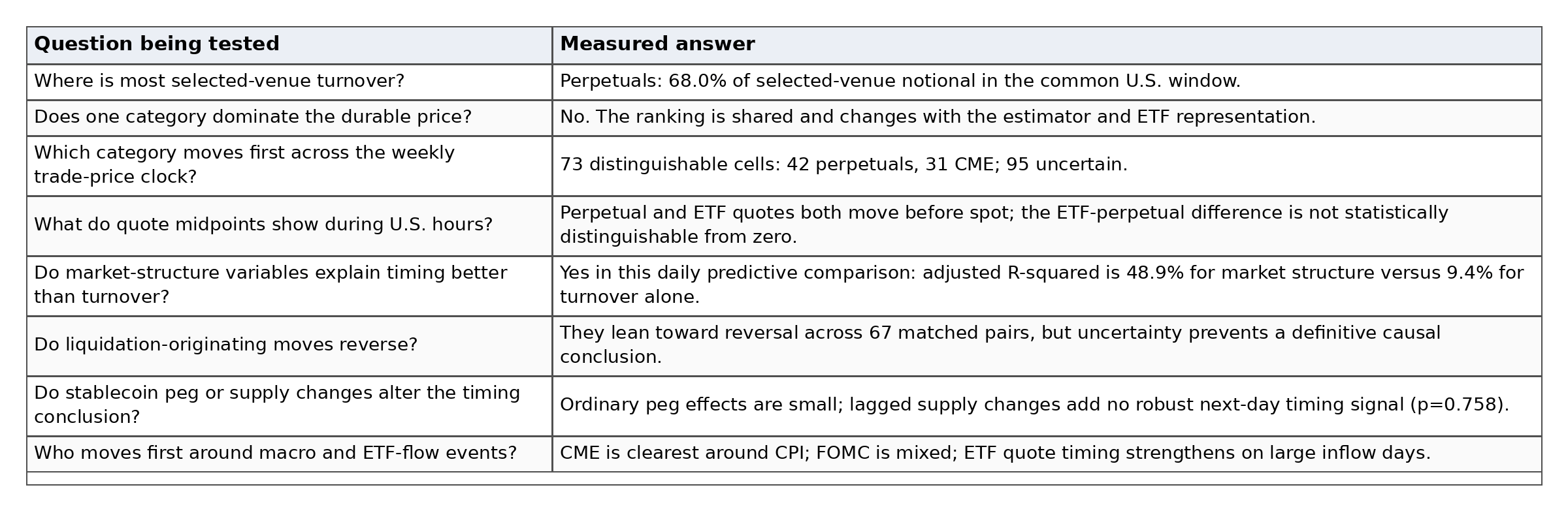
Source: SharpeEdge calculations. Definitions, equations, uncertainty and data limitations are documented below and in the technical appendix.

1. What price discovery means - and why these four markets
Price discovery is the process through which valuation-relevant information becomes incorporated into market prices. Bitcoin does not have one exchange or instrument that mechanically defines its value. Instead, several instruments represent claims on, exposure to, or ownership of the same economic asset. When those prices briefly disagree, arbitrage and hedging link them back to a common market-wide price.
The four categories were chosen through the same inclusion rule. Each had to provide: (1) a directly tradable Bitcoin-linked price; (2) economically material activity; (3) an observable arbitrage or hedging link to the other markets; and (4) sufficiently consistent minute-level history for a common comparison. The resulting evidence includes roughly 1.88 million minute observations for each major crypto series, 1.29 million CME quote records and 1.73 million ETF trade bars, supplemented by continuous quote summaries. Spot exchanges transfer actual Bitcoin ownership. Perpetual futures provide continuous leveraged exposure without an expiry date. CME futures are regulated, dated contracts used by traditional-finance participants. Spot Bitcoin ETFs are U.S.-listed shares linked to Bitcoin through creation, redemption and hedging. Options and over-the-counter trades matter, but options represent nonlinear payoffs and implied volatility rather than a directly comparable Bitcoin price, while OTC trades lack a transparent minute-by-minute record. Stablecoins affect funding and denomination but do not provide a separate Bitcoin price.
Price changes travel between the categories through concrete mechanisms. If a perpetual trades below spot, an arbitrageur can buy the perpetual and sell spot, narrowing the gap. If CME futures move after a macro release, dealers may hedge in spot or perpetuals. If an ETF trades away from the value of its Bitcoin holdings, authorized participants and market makers can create or redeem shares and hedge the exposure in spot or futures. These trades transmit the price movement; they do not prove that the first market possessed private information.
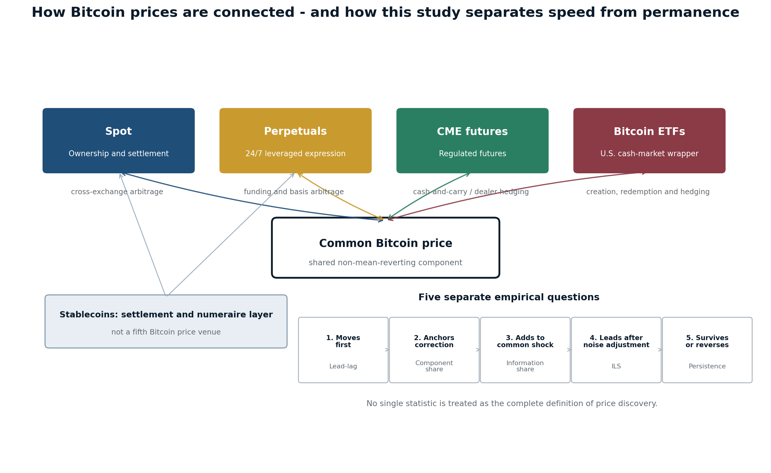
Figure 1. How the four price categories are connected and how the study separates temporal precedence, error correction, common-price innovation, noise-adjusted information leadership and persistence.
Source: SharpeEdge Capital conceptual framework. Stablecoins are shown as a settlement and numeraire layer rather than a separate Bitcoin price venue.

2. Volume is not information
Notional turnover is the gross dollar value of all executions during a period. It is calculated as trade price multiplied by traded quantity; for CME, contract volume is also multiplied by the standard five-Bitcoin contract size. Between the U.S. spot-ETF launch and 31 July 2026, the selected Binance and Bybit perpetual contracts processed $6.84 trillion during the common U.S. window. That was 68.0% of the four-category total, compared with 14.5% for five ETFs, 9.3% for CME futures and 8.3% for the selected spot venues.
Turnover is gross, not net. A trader who posts $10,000 of collateral to control a $100,000 leveraged perpetual position and then opens and closes it has generated $200,000 of notional turnover even though the capital committed was much smaller. A cash-and-carry trader can buy $1 million of spot Bitcoin and sell $1 million of futures, producing $2 million of turnover while carrying little net directional exposure. A liquidation engine can forcibly close positions, and arbitrageurs can then trade the same price movement across several venues. Each execution is real, but repeated transfer, hedging and forced trading are not the same as the arrival of new information.
The turnover percentages are an apples-to-apples comparison inside the exact set of instruments used in the price analysis, not an estimate of the entire global Bitcoin market. Every category is measured over the same dates and the same 10:00 a.m.-3:55 p.m. New York window. Spot combines Coinbase BTC/USD and Binance BTC/USDT; perpetuals combine Binance and Bybit; CME notional uses contract price, contract count and the five-Bitcoin multiplier; ETF notional uses share volume and VWAP across IBIT, FBTC, GBTC, ARKB and BITB. The percentages therefore answer: how is activity divided within the markets whose prices are compared here?
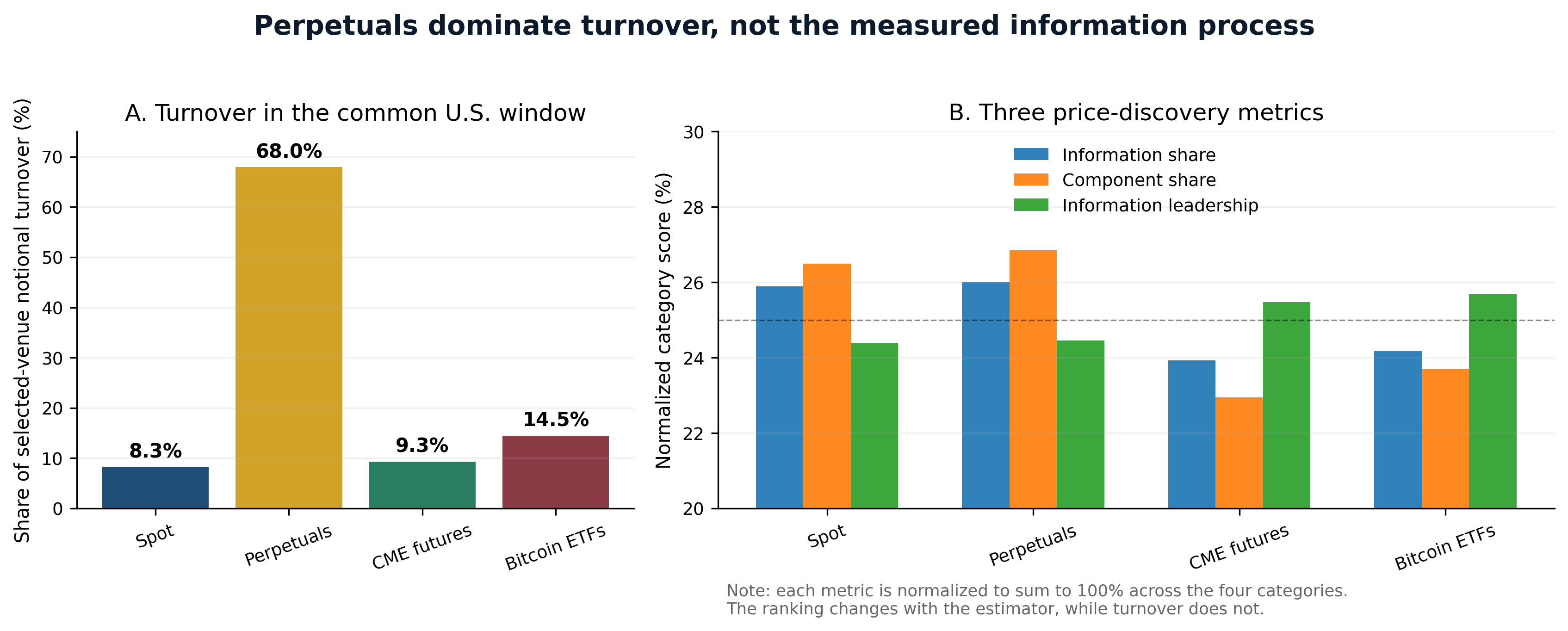
Figure 2. Selected-venue turnover shares and three normalized durable-price attribution scores in the post-ETF common U.S. window. Perpetuals account for almost 68% of turnover while all three attribution methods remain near one quarter per category.
Source: SharpeEdge Capital calculations from Binance, Bybit, Coinbase, CME/Databento and Alpaca SIP data. Common U.S. window: 10:00-15:55 ET, 11 January 2024-31 July 2026.
Why test turnover at all? Market commentary often assumes that the venue with the most trading should react first because informed traders and arbitrageurs may concentrate where activity is greatest. That is a plausible benchmark, not a claim that turnover causes speed. Leverage, hedging and repeated trading can break the link. Perpetuals’ turnover-to-Information-Leadership-Share ratio is 2.78; the ratios are 0.34 for spot, 0.37 for CME and 0.56 for ETFs. These are not efficiency grades; they show how far gross activity can diverge from estimated informational contribution.
3. How the study measures price discovery
No single statistic can observe “information” directly. The study therefore triangulates five distinct questions. A “price-discovery score” in this article means a category’s normalized share under a named method; it is not a composite grade invented by the study. Each method is reported separately because it answers a different question.
Table 2. Plain-language guide to the five measurement dimensions
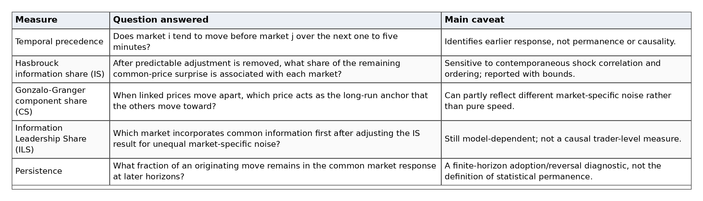
Information-share methods focus on unexpected changes because a price movement that can already be predicted from recent returns or an existing cross-market gap is not fresh information. The residual surprise - the part the model could not predict - is the portion that can update the common price. ILS adjusts IS with Component Share: it rewards a market whose surprises enter the common price early, but discounts an apparent lead that is mainly associated with temporary market-specific noise.
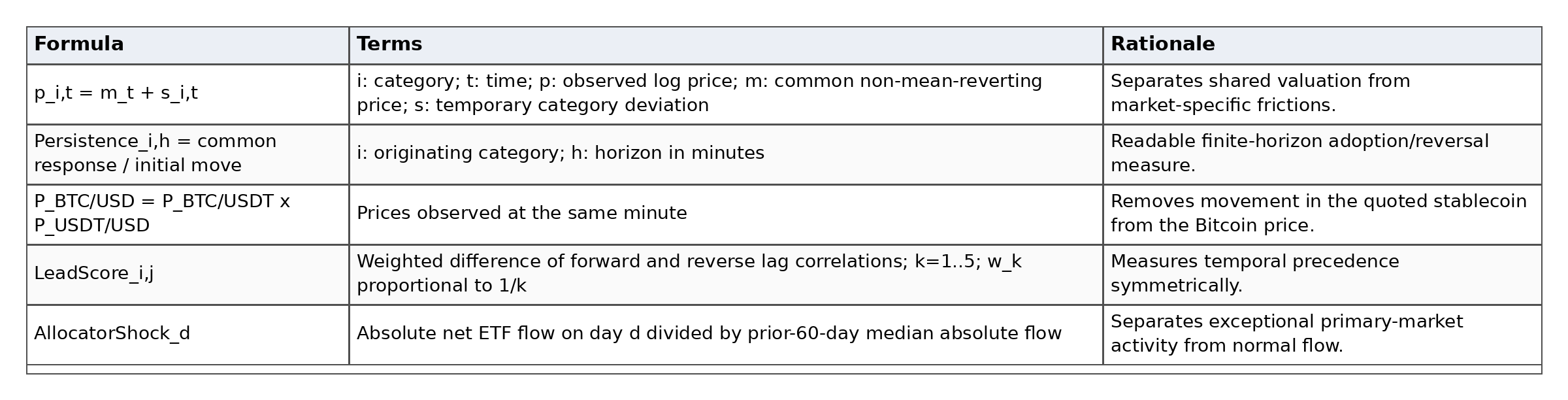
The common-price idea can be written as:

The subscript i identifies one of the four market categories - for example the spot composite, the perpetual composite, CME futures or Bitcoin ETFs - and t identifies time. p_i,t is the natural logarithm of the observed price in that category. Log prices put a 1% move on the same scale whether the instrument is a $60,000 Bitcoin price or a much lower-priced ETF share. m_t is the unobserved common Bitcoin price: the shared trend that does not systematically reverse. s_i,t is the temporary category-specific deviation caused by basis, inventory pressure, market frictions or noise. The equation is a conceptual decomposition; vector error-correction models (VECMs: models that estimate how linked prices close temporary gaps while sharing a common long-run trend) infer how observed prices adjust around that common trend.
Persistence is calculated as:

Here i is the originating category and h is the horizon, such as 5, 30 or 120 minutes. A value of 1 means the common market price has retained the full initial move; a value below 1 indicates partial reversal; a value above 1 indicates continuation. Persistence is evaluated as a path, not assumed to decline smoothly. A move can dissipate and later reappear as additional information arrives or other markets reopen.
Hasbrouck developed Information Share [1], Gonzalo and Granger developed the permanent-component logic behind Component Share [2], and Putnins developed Information Leadership Share [3]. This study applies them through five transparent choices. The daily pairwise tournament compares each category with the other three on every eligible day and then averages those three scores. The availability-aware weekly map includes a market only when it is open. The symmetric persistence analysis uses the same shock-selection rules and horizons for every category. The stablecoin correction converts USDT-quoted prices into dollar-equivalent prices. The event modules repeat the timing and persistence tests around macro releases, ETF-flow regimes, liquidation episodes and the CME weekend schedule change.
How to read uncertainty and model fit
A 95% bootstrap interval is built by repeatedly resampling the relevant days or event pairs and recalculating the statistic. It is an empirical uncertainty range: if it crosses zero, the sign of the estimated difference is not stable across resamples. A p-value asks how often a result at least as extreme would arise under a specified no-effect assumption; it is not the probability that the no-effect assumption is true. The common 5% threshold is a convention, not a proof boundary, so results near it are described cautiously.
Adjusted R-squared is the share of in-sample variation explained after penalizing the model for adding predictors. Out-of-sample R-squared compares prediction errors on held-out days with a constant-mean benchmark. A value of 0.321 means about 32.1% lower squared error than that benchmark; a negative value means the model predicts worse than the benchmark. A basis point is 0.01 percentage point. When the article says two markets are statistically tied, it means the uncertainty interval for their difference includes zero.
4. What previous studies found - and why they disagree
The literature does not offer one stable Bitcoin price-discovery winner. That is not simply academic inconsistency: the studies examine different market structures, periods, instruments, data frequencies and estimators.
Table 3. Selected Bitcoin price-discovery literature and sources of disagreement
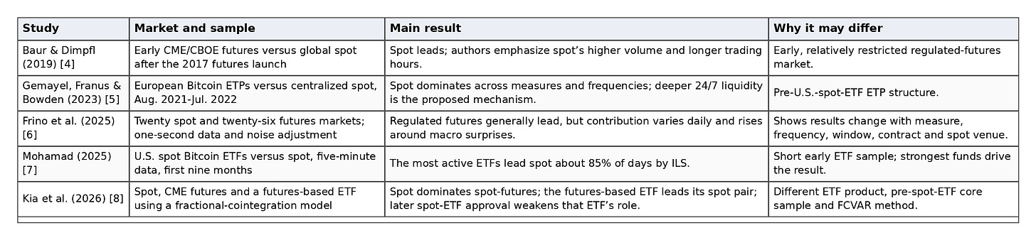
Five factors reconcile much of the apparent contradiction. First, market structure changed: a thin early futures market is not the same as the post-2024 ETF ecosystem. Second, trading hours and liquidity differ across products. Third, one-second data can resolve reactions that one-minute or five-minute bars merge together. Fourth, IS, CS, ILS and fractional-cointegration models do not estimate identical objects. Fifth, results depend on which spot exchanges, futures contracts and ETFs represent each category. Frino et al. explicitly identify metric, sampling frequency, modeling window, futures contract and spot venue as sources of conflicting conclusions [6].

5. Data construction, normalization and claim limits
The full sample runs from 1 January 2023 through 31 July 2026; the four-category post-ETF analysis begins on 11 January 2024. The evidence comprises approximately 1.88 million one-minute observations for each major crypto price series, 1.29 million CME sampled best-bid-and-offer records, 857,635 CME trade bars, 1.73 million ETF trade bars, 664 daily ETF-flow observations, 376,571 five-minute derivatives-metric observations, 8,431 venue-day quote summaries, 20,881 direct-liquidation active minutes, 1,484,149 USDC/USD minute bars and 2,616 USDT/USDC daily supply observations.
Why geometric means are used
Spot is the geometric mean of Coinbase BTC/USD and a dollar-adjusted Binance BTC/USDT price; perpetuals use the same construction for Binance and Bybit. For two positive prices P1 and P2, the geometric mean is the square root of P1 x P2. It is the price that lies the same proportional distance from both inputs, so each venue receives equal percentage weight. For example, prices of $60,000 and $60,600 have an arithmetic mean of $60,300 and a geometric mean of about $60,299.25 - virtually identical, but the geometric mean is exactly consistent with percentage-based price comparisons. In this dataset the choice is economically immaterial: the median absolute arithmetic-versus-geometric difference is below 0.00002 basis points for both composites.
Trade prices and quote midpoints answer different questions
A trade price is the price of an executed transaction. It is the appropriate input for turnover and for the primary transaction-price analysis. A quote midpoint is halfway between the best available bid and ask; it represents the market’s current quoted valuation and also provides the bid-ask spread and quoted size. The study does not replace one with the other. It reports trade-price timing as the primary full-market clock and uses quote midpoints as a complementary timing and execution-quality test. IBIT is the primary ETF trade-price series because it has the densest active-minute coverage; a five-fund median-return composite checks whether the durable-price result belongs to the ETF category rather than one fund. A separate five-fund quote composite uses one-minute bid and ask observations for IBIT, FBTC, GBTC, ARKB and BITB, with fill-forward disabled.
Stablecoin conversion and CME rolls
BTC/USDT is converted to a dollar-equivalent price using:

P_BTC/USDT,t is the Bitcoin price quoted in Tether at time t; P_USDT/USD,t is the dollar value of one USDT. USDT/USD is carried forward for no more than five minutes. Kraken USDC/USD is analyzed separately as a peg and tail-risk robustness series. The available price universe does not include a complete BTC/USDC history, so the article does not rank a BTC/USDC venue; it compares USDC and USDT peg behavior and stablecoin supply conditions instead.
CME futures expire. The continuous series switches among monthly contracts identified by instrument ID. Returns on transition minutes are set to missing, and the within-day futures-spot spread is demeaned in common-price models. That prevents a roll jump from being mislabeled as Bitcoin information.
Sampled depth, trade size and liquidation records
The order-book and liquidation evidence is deliberately sampled. Quote and trade files cover 1 January and 1 July in each year from 2023 through July 2026 (eight days); top-five depth covers 1 January of 2023-2026 (four days); direct liquidation files cover the first day of every month (43 days). Those dates are used because the provider makes the first day of each month available for historical research without a full commercial history. The sample supports mechanism checks - spreads, trade size, depth and forced-flow reversal - but it is not a continuous estimate of Level-2 conditions on every day.
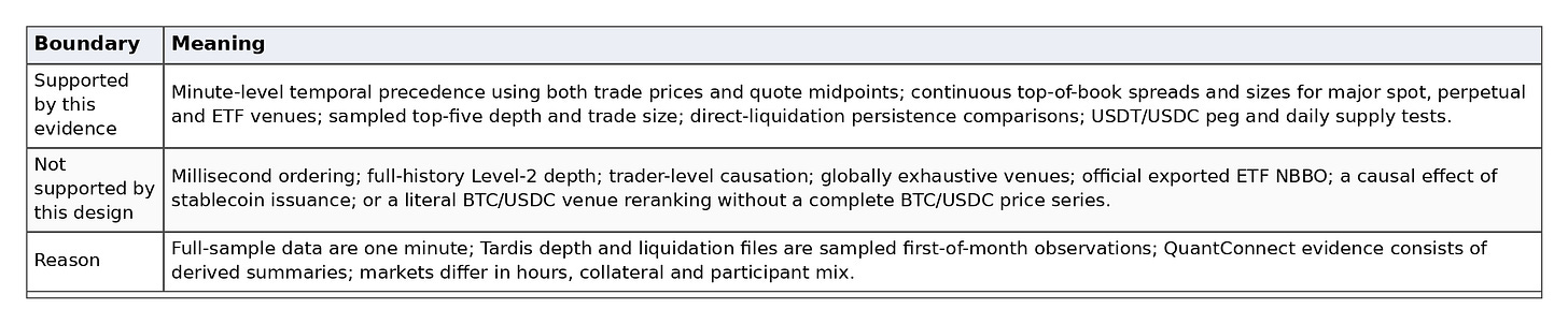
What the evidence can and cannot establish
Table 4. Scope of the evidence and remaining boundaries
6. The durable-price ranking does not survive the estimator
The durable-price analysis uses a vector error-correction model (VECM), which is designed for prices that represent the same underlying asset and therefore share a long-run relationship even though temporary gaps appear. For each pair, the model asks two things at once: how recent price changes carry forward, and which price adjusts when the pair was out of line in the previous interval. That correction behavior reveals the long-run anchor and the shocks that update the common price. Hasbrouck Information Share attributes the variance of the unanticipated common-price shock; Component Share identifies the price that the other tends to adjust toward; Information Leadership Share combines the two and discounts an apparent lead associated with temporary market-specific noise.
The model uses 5-minute log prices. Five-minute sampling reduces one-minute quote and transaction noise, aligns markets with different trading activity, and still leaves about 72 observations in a normal six-hour common window - enough to estimate a daily adjustment model. Log prices are used because their differences are percentage returns: a 1% move has the same meaning for Bitcoin spot, a futures price and an ETF share even though their dollar levels differ. For every eligible day and pair of categories, the study estimates the VECM, averages each category’s three pairwise scores and normalizes the four category scores to 100%. This pairwise tournament avoids forcing one unstable four-market model onto every day.
The ILS tournament gives Bitcoin ETFs 25.68%, CME 25.47%, perpetuals 24.46% and spot 24.38%. Weekly-block bootstrap intervals place ETF at 25.22%-26.16% and CME at 25.20%-25.92%. The point estimate favors ETFs, but the CME-ETF difference spans zero. Spot and perpetuals are also statistically indistinguishable.
Hasbrouck IS and Component Share point the other way: spot and perpetuals receive slightly more than one quarter, while CME and ETFs receive slightly less. ILS reverses the order because it explicitly adjusts for relative noise. Pairwise residual innovations are almost perfectly correlated and Hasbrouck ordering bounds are extremely wide. In a market where prices reprice nearly together, a small modeling choice can determine the ordinal ranking.
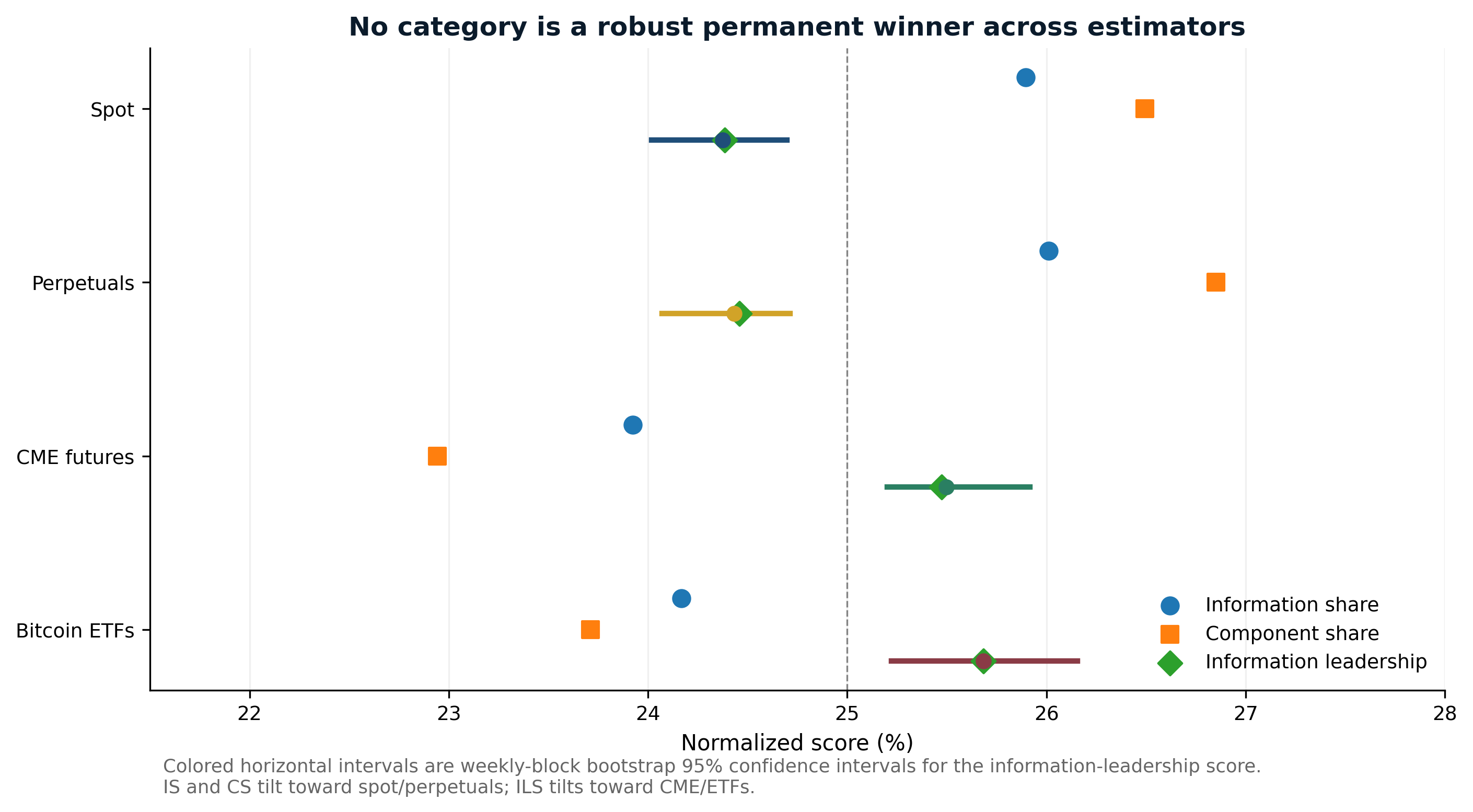
Figure 3. Normalized category scores under Hasbrouck Information Share, Component Share and Information Leadership Share. Colored horizontal intervals are weekly-block bootstrap confidence intervals for ILS.
Source: SharpeEdge Capital daily pairwise VECM estimates. The scores are normalized category-tournament outputs, not raw shares from one four-market structural model.
Replacing IBIT with the five-fund return composite lowers the ETF score from 25.68% to 24.47% and raises spot to 25.12%, while CME remains 25.48%. Excluding 14:00-15:59 UTC, a conservative window around benchmark and settlement-sensitive activity, leaves the four scores near 25%. The apparent ETF edge is therefore not a robust category-wide permanent-price result.
7. Which market moves first changes around the clock
For every category pair, the temporal-precedence statistic compares the correlation of market i now with market j one to five minutes later against the reverse correlation. Shorter lags receive more weight. A positive category score means that its current return contains more information about the others’ next few minutes than the reverse. It is a timing measure, not a permanent-price or causal claim.

r_i,t is the one-minute log return of category i at time t; k is the lead in minutes; w_k is proportional to 1/k, so the nearest minute receives the greatest weight. A heat-map cell is colored only when the top category exceeds the runner-up by at least 1.96 pooled standard errors across weekly estimates. The value 1.96 is the usual normal-approximation cutoff for a 95% pointwise confidence rule - roughly two standard errors - and is used as a display filter so uncertain cells remain gray. It is not a universal proof threshold or a correction for all 168 comparisons. At a looser 90% cutoff, 85 cells are colored (48 perpetuals and 37 CME); at a stricter 99% cutoff, 49 remain (26 and 23). The category pattern is unchanged even though the number of colored cells changes.
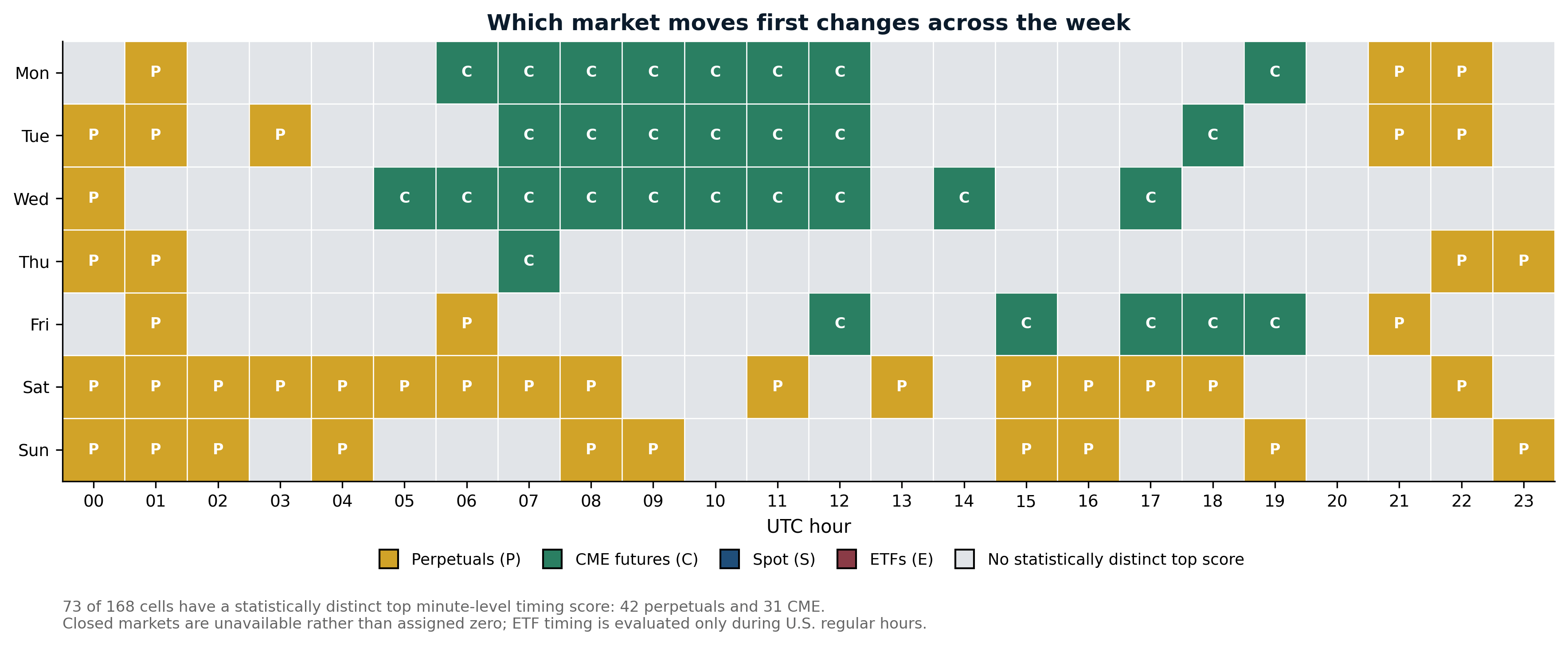
Figure 4. Availability-aware hour-of-week map of the statistically distinguishable top trade-price temporal-precedence score. Gray cells indicate that no category can be cleanly ranked; P is perpetuals and C is CME futures.
Source: SharpeEdge Capital weekly lead-lag estimates, post-ETF sample. ETF observations enter only during U.S. regular hours. Times are UTC.
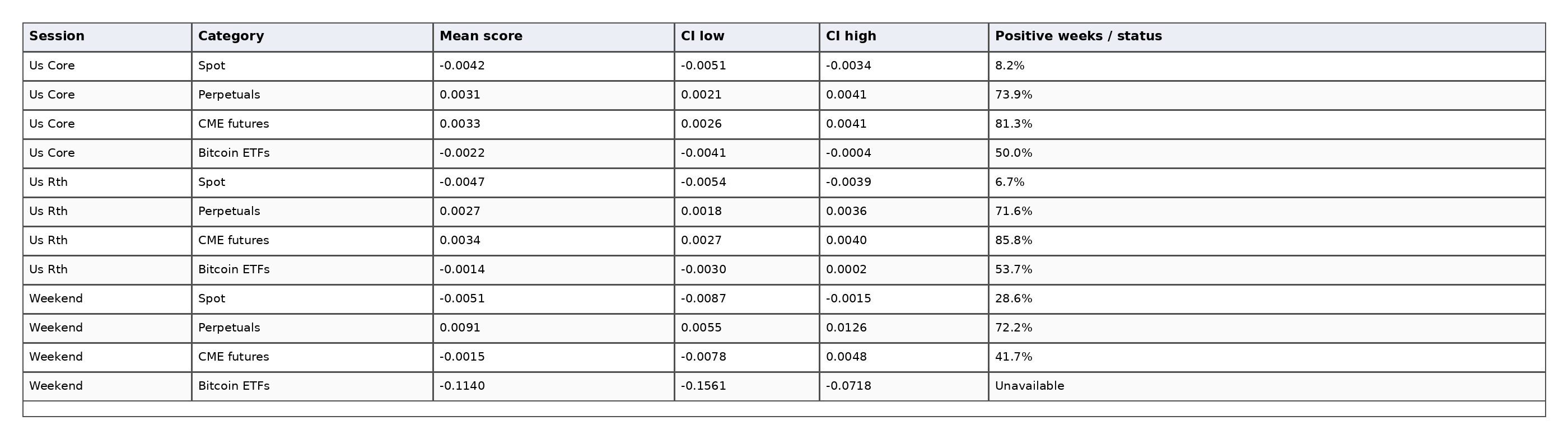
Only 73 of 168 cells have a statistically distinguishable top trade-price score; 95, or 56.5%, remain tied or too uncertain. Among the distinguishable cells, perpetuals account for 42 and CME for 31. During the common U.S. window, CME’s mean trade-price score is 0.0033 and perpetuals’ is 0.0031; their intervals overlap. On weekends, perpetuals’ score is 0.0091 with an interval above zero.
Trade prices and quote midpoints provide complementary timing evidence
The transaction-price clock and the quote-midpoint comparison are both retained; one is not substituted for the other. Trade prices show the sequence of actual executions. Quote midpoints show how the best bid and ask are being revised. During U.S. hours, the five-fund ETF quote composite leads spot by 0.0064, with a 95% interval of 0.0044 to 0.0084. Perpetual quotes lead spot by 0.0061, with a 95% interval of 0.0051 to 0.0071. The ETF-over-perpetual point estimate is 0.0009, but its interval (-0.0011 to 0.0028) spans zero. The defensible conclusion is that ETF and perpetual quotes both reprice before spot and cannot be cleanly ranked against each other.
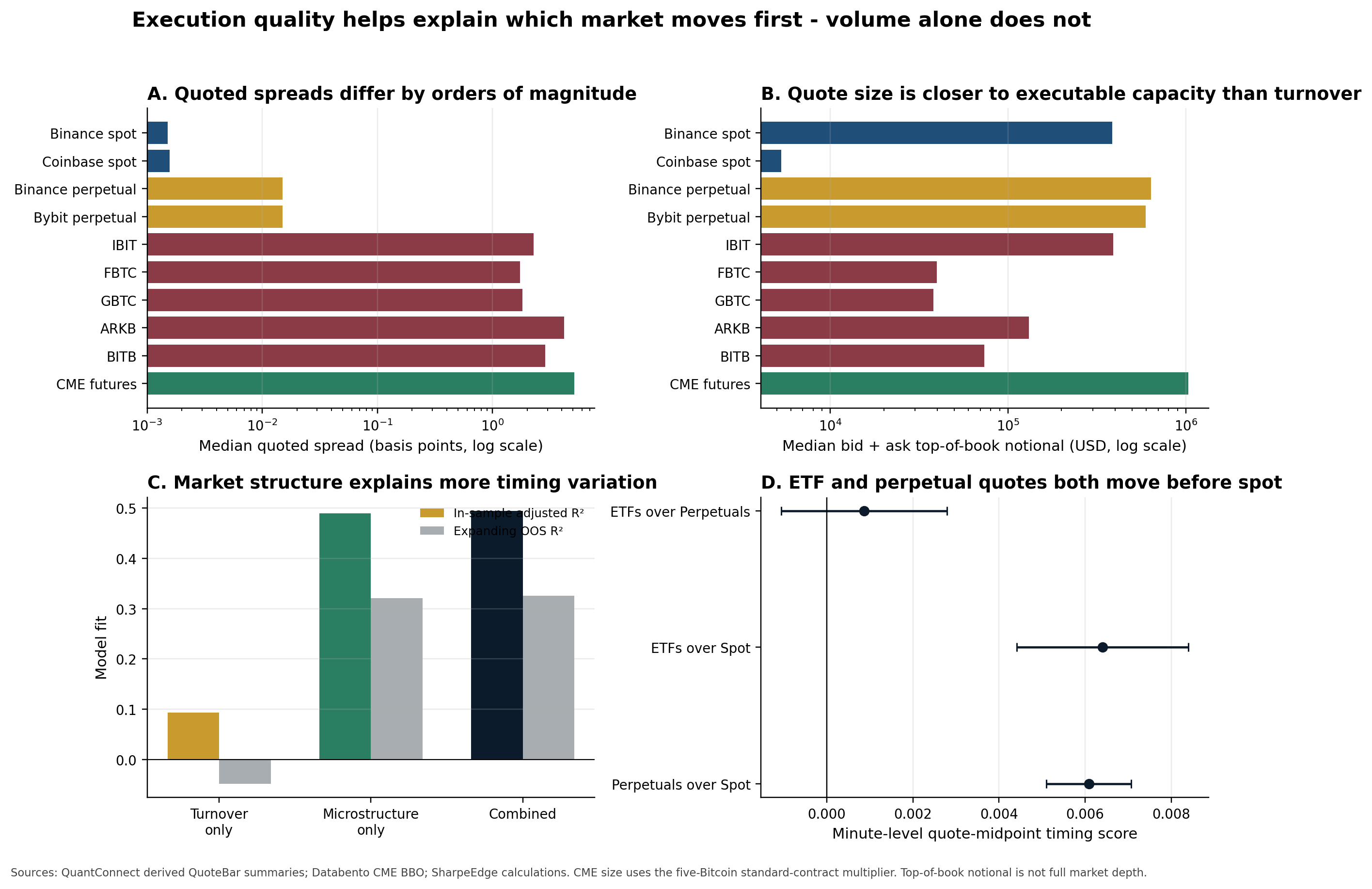
Figure 5. Execution-quality and quote-timing evidence. Panels compare venue spreads, top-of-book quote notional, turnover-only versus microstructure model fit, and U.S.-window quote-midpoint temporal precedence.
Sources: QuantConnect derived QuoteBar outputs; Databento CME BBO; SharpeEdge calculations. Top-of-book notional is not full market depth; CME notional uses the five-Bitcoin standard-contract multiplier.
Market structure explains more than turnover
This is a daily linear prediction exercise, not a causal model. The outcome is the perpetual-over-spot quote lead: a positive value means perpetual quotes tend to precede spot quotes that day. The turnover-only benchmark asks whether the relative share of perpetual turnover is enough to predict that score. The rationale is the common industry claim that the most heavily traded market should process information fastest; the benchmark tests that claim rather than assuming it. The market-structure model instead uses the perpetual-versus-spot differences in top-of-book notional, quoted spread, absolute imbalance, return volatility and quote inactivity. The turnover benchmark has adjusted R-squared 0.094 and out-of-sample R-squared -0.048. The market-structure model reaches 0.489 in sample and 0.321 out of sample; the combined model reaches 0.495 and 0.325. In plain terms, the market-structure model explains about half of the observed daily variation and cuts held-out squared prediction error by about one-third. That is meaningful for a noisy market-timing outcome, but it is not close to a complete forecast and does not prove causation.
In the combined standardized model, larger perpetual top-book notional is positively associated with earlier perpetual movement (coefficient 0.17, p=0.003); higher relative quote inactivity is strongly negative (-0.59, p<0.001); and the volatility ratio is strongly positive (0.36, p<0.001). The spread-gap coefficient is not significant. The result is not simply “the tightest spread wins”; active quote capacity and information flow matter more.
Sampled order books support the same channel
In the sampled order-book data described in Section 5, the eight quote-and-trade days and four depth days show clear differences in transaction size and displayed capacity. Median average trade notional is about $520 on Binance spot and $410 on Kraken spot, versus $3,333 on Binance perpetuals and $3,678 on Bybit perpetuals. Median bid-plus-ask depth across the top five levels is about $414,000 for Binance spot, $987,000 for Binance perpetuals and $822,000 for Bybit perpetuals. These observations support a liquidity mechanism, but the sampled dates are not a continuous full-history depth panel.
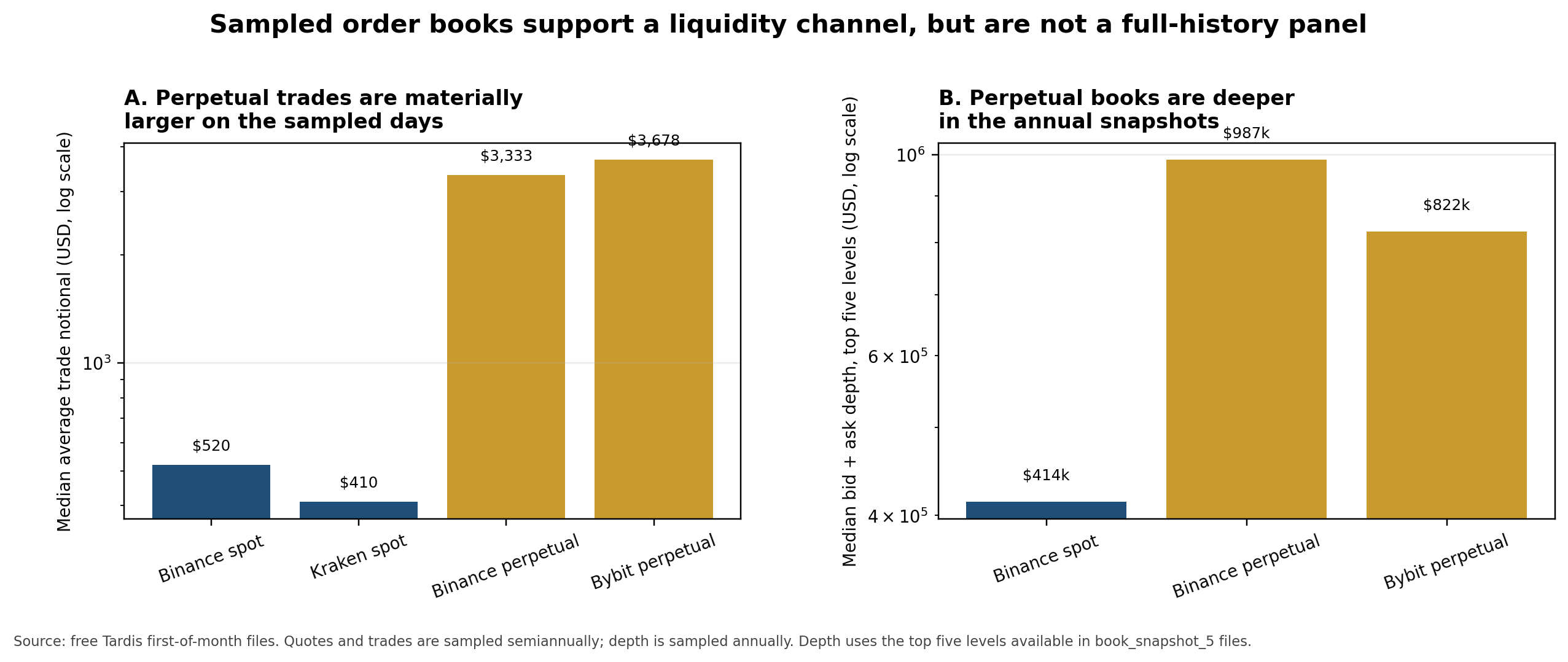
Figure 6. Sampled average trade notional and top-five order-book depth for spot and perpetual venues.
Source: free Tardis first-of-month files. Quotes and trades are sampled semiannually; depth is sampled annually. Depth uses the top five levels available in book_snapshot_5 files.
8. Fast does not always mean adopted
The persistence analysis starts with large, category-specific one-minute return shocks selected symmetrically across categories. It then measures the common cross-category response after 1, 5, 30 and 120 minutes. The path is allowed to be non-monotonic: a move can partially reverse, later resume, or be overtaken by new information. That is why the article reports the full curve rather than one arbitrary cutoff.
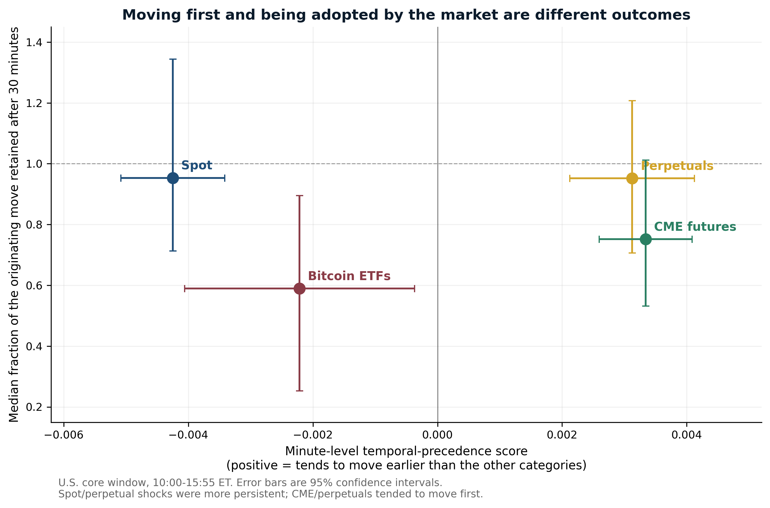
Figure 7. Temporal precedence versus 30-minute persistence in the common U.S. window. Horizontal error bars show weekly uncertainty in the timing score; vertical bars show bootstrap uncertainty in persistence.
Source: SharpeEdge Capital calculations. Positive x-axis values indicate earlier movement; a y-axis value of one means the common price retained the full initial move.
At 30 minutes, spot and perpetual shocks are most fully adopted: 0.95 and 0.95. CME-originating shocks retain 0.75; ETF shocks retain 0.59. Confidence intervals are wide, especially for ETFs, so these are median paths rather than deterministic rules.
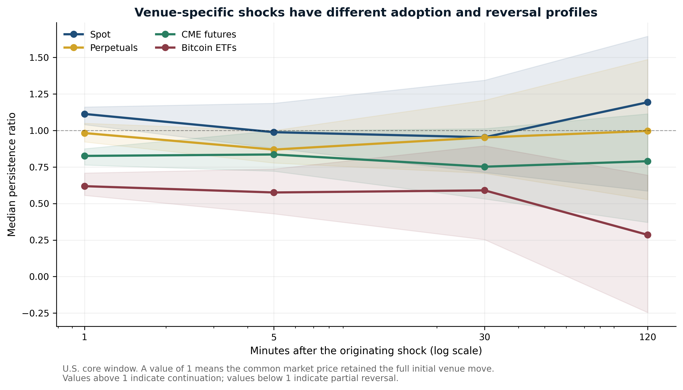
Figure 8. Median adoption of category-originating shocks after 1, 5, 30 and 120 minutes in the common U.S. window. The curves are deliberately allowed to fall and then recover.
Source: SharpeEdge Capital event-based persistence estimates. Shaded regions are 95% bootstrap intervals.
The non-monotonicity is economically meaningful. Spot moves from 1.11 at one minute to 0.95 at 30 minutes and back to 1.19 at 120 minutes. Perpetuals move from 0.98 to 0.87, then recover to 1.00. CME moves from 0.83 to 0.75 and back to 0.79. ETF persistence declines from 0.62 to 0.29. These paths show why “what remains after 30 minutes” is a readable diagnostic, not the definition of permanence.
Direct liquidation records provide the stronger test
The direct-liquidation sample contains $1.16 billion of Binance and Bybit liquidations across 43 first-of-month days. The comparison selects the top 1% of liquidation minutes, requires the perpetual price to move at least three basis points in the direction implied by the forced flow, and separates events by 30 minutes. Each event is matched with a same-day price shock of similar initial size that contains no recorded liquidation in that minute, producing 67 pairs. This matched design asks whether forced-flow shocks behave differently from otherwise similar moves; it is the stress comparison referred to in the executive summary.
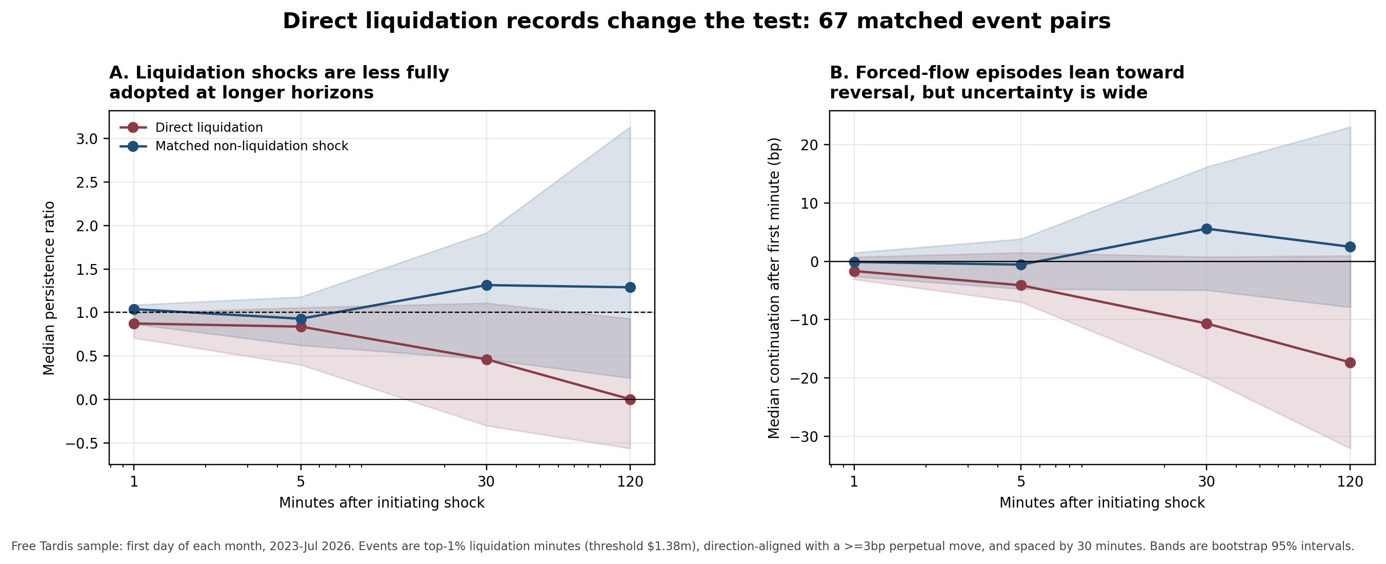
Figure 9. Persistence and continuation after direct-liquidation shocks versus matched non-liquidation shocks.
Source: SharpeEdge Capital calculations from free Tardis Binance and Bybit liquidation files and the perpetual composite. Bands are bootstrap 95% intervals; sampled days are the first day of each month.
Direct-liquidation shocks have median persistence of 0.87 after one minute, 0.84 after five minutes, 0.46 after 30 minutes and 0.00 after two hours. Matched controls are 1.04, 0.93, 1.31 and 1.29. At two hours, liquidation events show 61.2% reversal versus 43.3% for controls. The median continuation difference is -19.8 basis points. A bootstrap - repeated resampling of the matched pairs - gives a 95% interval of -49.7 to -0.0 basis points, barely excluding zero. A Mann-Whitney rank test, which asks whether the entire liquidation distribution tends to be lower, gives p=0.099; under equal distributions, a rank difference this large or larger would occur about 9.9% of the time. Because the two methods disagree at the margin and the sample covers selected days, the result is economically suggestive rather than definitive causal proof.
9. Information-arrival regimes
9.1 Consumer prices and Federal Reserve decisions
The event sample includes 30 U.S. Consumer Price Index (CPI) releases and 21 Federal Open Market Committee (FOMC) decisions, aligned to the official public-release minute. CPI measures consumer-price inflation and is normally released before the U.S. ETF regular session; the FOMC is the Federal Reserve committee that announces monetary-policy decisions, normally at 2:00 p.m. New York time.
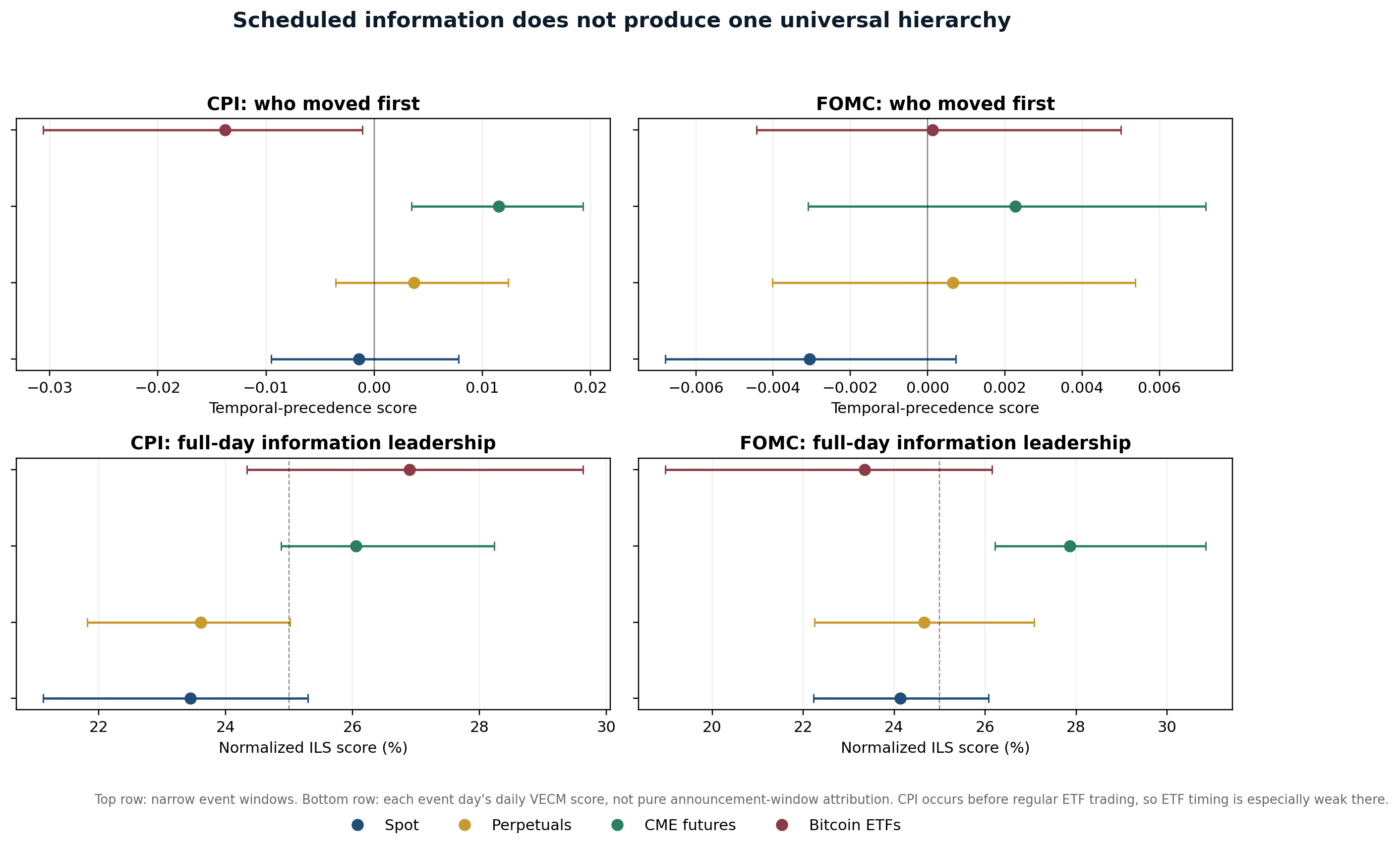
Figure 10. Minute-level temporal-precedence scores and full-day Information Leadership Share scores around CPI and FOMC events. The legend maps blue to spot, gold to perpetuals, green to CME futures and burgundy to Bitcoin ETFs.
Source: SharpeEdge Capital calculations; event timestamps from the U.S. Bureau of Labor Statistics and Federal Reserve. Top panels use narrow event windows. Bottom panels use each event day’s daily VECM and are not pure announcement-window attribution.
CME is the clearest first mover around CPI. Its narrow-window temporal score is 0.0115, its 95% interval remains above zero, and it has an 87.2% bootstrap probability of being the highest. FOMC timing is less hierarchical: CME has the highest point estimate, but the intervals for CME, perpetuals and ETFs overlap zero and one another. Full-day FOMC models give CME a 27.9% ILS score and a 96.3% probability of being the highest, but that is an event-day association rather than proof that CME alone originated the announcement-window permanent shock.
Did the event moves persist?
The analysis also measures the common-market response relative to the initial one-minute move. Events with an initial common move below five basis points are excluded so that ratios are not dominated by a near-zero denominator.
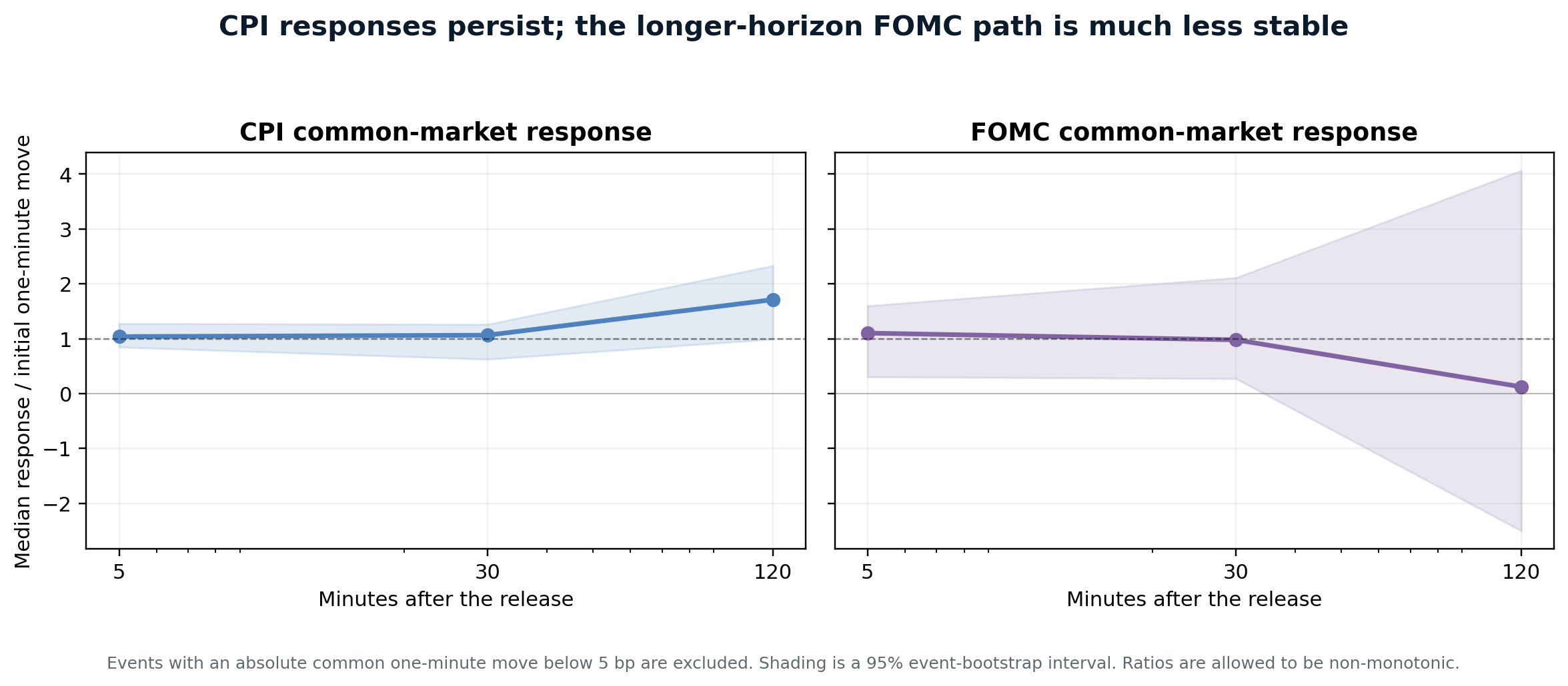
Figure 11. Common-market persistence after CPI and FOMC announcements. Ratios may be non-monotonic; shaded regions are 95% event-bootstrap intervals.
Source: SharpeEdge Capital calculations from the four category return series. Twenty-eight CPI events and twenty FOMC events pass the five-basis-point initial-move filter.
Table 6. Common-market persistence after scheduled announcements

CPI responses are close to fully retained at 5 and 30 minutes and continue at 120 minutes, although the long-horizon interval is wide. FOMC responses are close to one through 30 minutes but become highly unstable by 120 minutes: the median is near zero, the interval spans large continuation and reversal, and only 55% remain in the initial direction. The FOMC path illustrates why persistence can dissipate and reappear rather than decay smoothly.
The quote data add an execution-quality check around the announcements. Median crypto quoted spreads remain extremely small before and after both event types: roughly 0.0013 basis points for the spot composite and 0.013 basis points for the perpetual composite, with economically negligible median changes. At FOMC, the five-fund ETF quote spread rises from about 2.43 to 2.70 basis points, but the median event-level change is only 0.01 basis points. CPI occurs before the ETF regular session, so no comparable ETF quote window is available.

9.2 Allocator flows
ETF secondary-market turnover and primary-market allocator flow are not the same variable. ETF shares can trade between investors or market makers without changing the fund’s shares outstanding. Net creations and redemptions are closer to new allocator demand, but their exact intraday information time is not directly observed. The study therefore classifies days using lagged baselines rather than inserting an end-of-day flow estimate into a minute-level regression.

d indexes the trading day. The numerator is the absolute net creation or redemption estimate across the U.S. Bitcoin ETFs. The denominator is a lagged 60-day median, preventing the current day from defining its own threshold. The top decile is classified as a large primary-flow day.
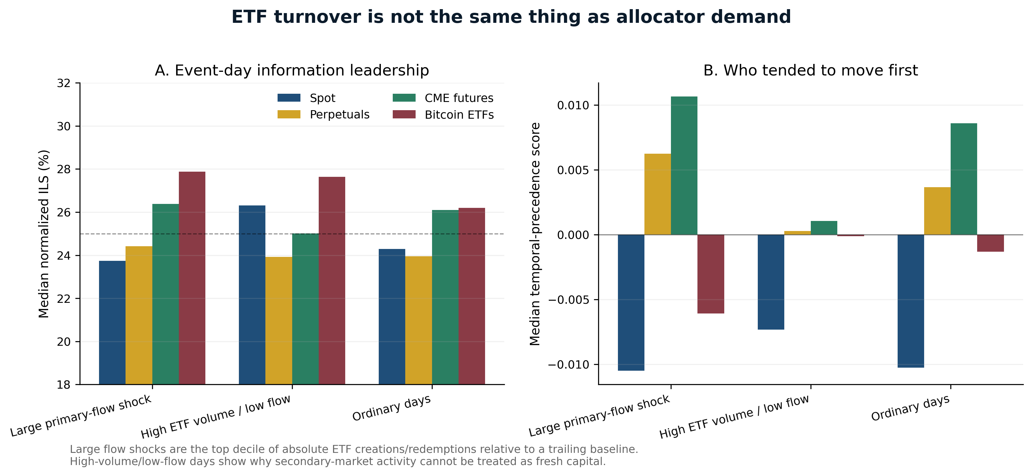
Figure 12. Information Leadership Share and temporal-precedence scores on large primary-flow days, high-volume/low-flow days and ordinary days. ILS measures noise-adjusted contribution to the common price; the temporal score measures who tends to move earlier.
Source: SharpeEdge Capital calculations from Alpaca SIP ETF bars and Farside daily flow estimates. Flow classifications use lagged baselines.
On large absolute-flow days, median normalized ILS scores are 23.7% for spot, 24.4% for perpetuals, 26.4% for CME and 27.9% for ETFs. CME and perpetuals still tend to move first: their median temporal scores are 0.0106 and 0.0062. Eleven high-volume/low-flow days produce a median ETF ILS of 27.6%, slightly above the large-flow median. High ETF trading is therefore not a reliable proxy for fresh allocator demand.
Quote-midpoint timing adds a more nuanced allocator result. On large inflow days, the ETF quote composite has median net lead 0.0049, compared with 0.0014 for perpetuals. On large outflow days, ETF quote timing falls to -0.0003 while perpetuals rise to 0.0039. High-volume/low-flow days still show positive ETF quote timing, confirming that fast ETF repricing is not the same as new primary-market demand.
9.3 CME weekend availability
Beginning at 4:00 p.m. Chicago time on 29 May 2026, CME made its cryptocurrency futures and options continuously available through weekends, apart from a scheduled weekly maintenance period [12]. The change did not create a new contract; it expanded the trading schedule of the existing regulated futures. It was also not the first regulated U.S. 24/7 crypto-futures market, because Coinbase Derivatives had already introduced continuous trading in May 2025 [11].
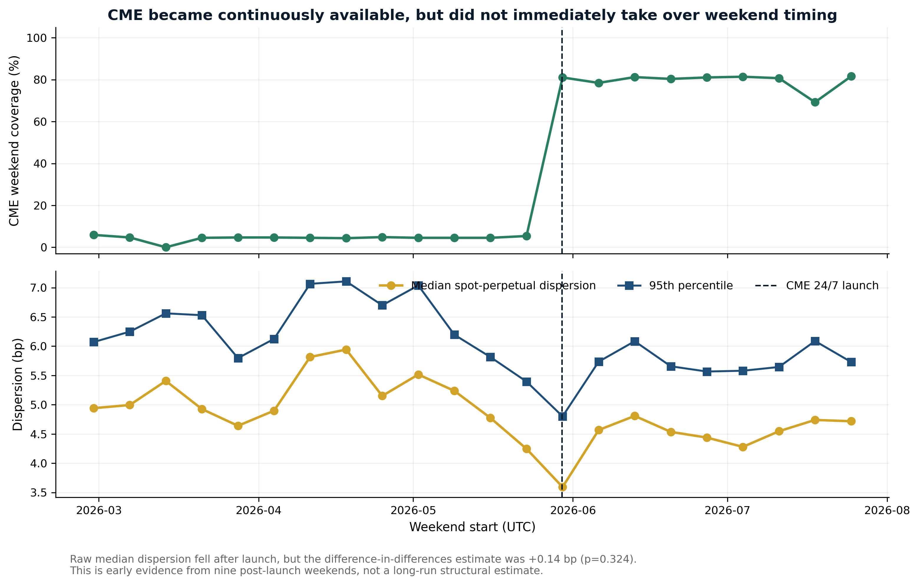
Figure 13. CME weekend quote coverage and spot-perpetual price dispersion before and after the 29 May 2026 schedule expansion.
Source: SharpeEdge Capital calculations. The post period contains nine weekends; all conclusions are preliminary.
CME weekend coverage rises from 4.3% to 79.5%. Raw median spot-perpetual dispersion falls from 5.09 to 4.50 basis points. But the difference-in-differences coefficient is +0.14 basis points with p=0.324. This means the weekend improvement was not statistically different from the contemporaneous weekday change. Perpetuals still move before spot and CME in the first nine post-launch weekends.

10. Stablecoins are numeraires, funding variables and tail risks - not a fifth venue
The sample contains full-period USDT/USD and USDC/USD minute series. USDT has exact minute coverage of 99.6% and 99.9% with a five-minute carry limit. USDC has exact coverage of 78.8% and 98.7% after the same limit. Normal USDC deviations are tighter: its 1st-to-99th percentile range is -5.0 to 2.0 basis points, versus -16.0 to 17.4 for USDT.
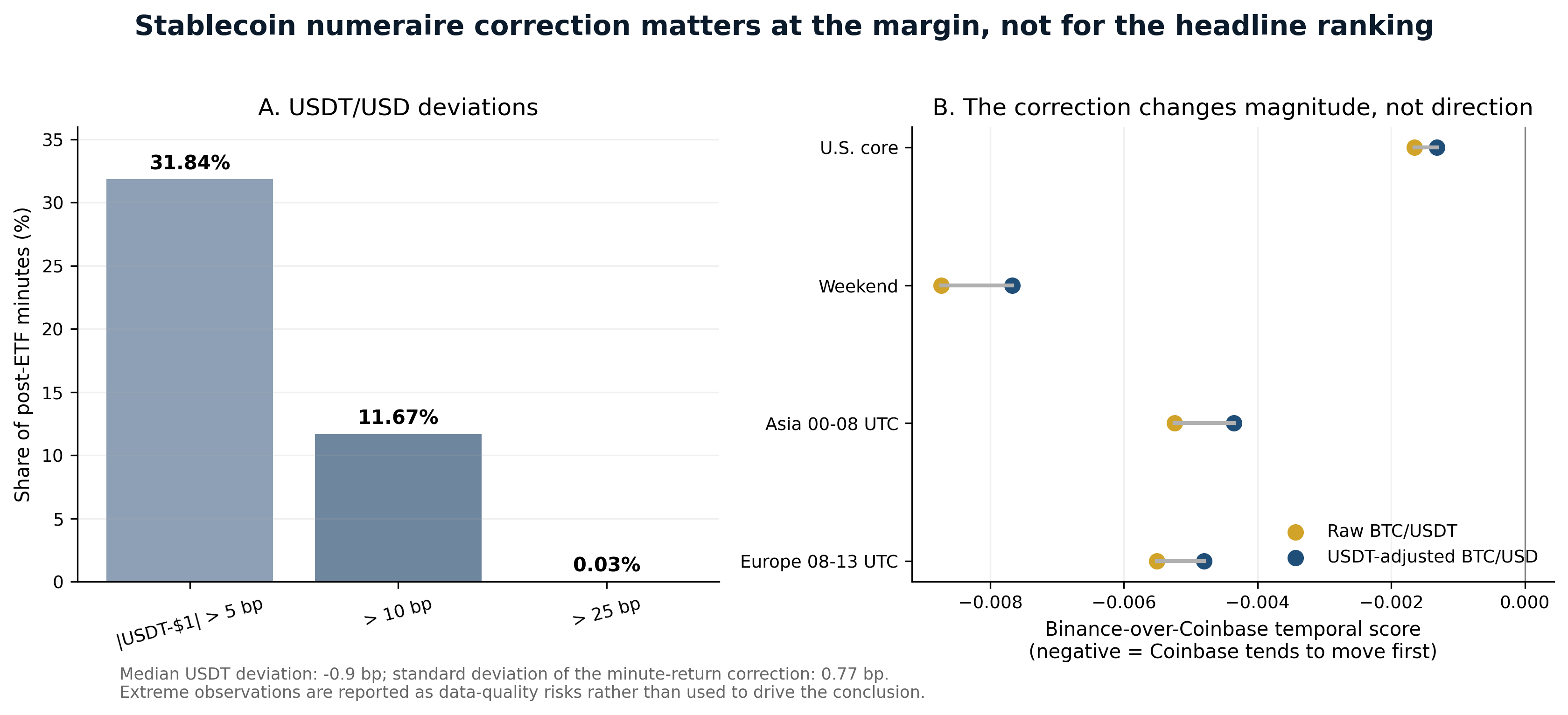
Figure 14. USDT/USD deviation frequency and its effect on Binance-versus-Coinbase trade-price temporal scores.
Source: SharpeEdge Capital calculations from Coinbase USDT/USD and BTC/USD and Binance BTC/USDT. Extreme illiquid observations are treated as data-quality risks.
The full-sample USDT correction attenuates the apparent Coinbase lead over Binance but does not reverse it. In the common U.S. window, the Binance-over-Coinbase trade-price score moves from -0.00165 in raw BTC/USDT to -0.00132 after conversion; on weekends it moves from -0.00873 to -0.00767.
USDC is normally tighter, but its March 2023 depeg created the larger tail
On 10 March 2023, Silicon Valley Bank was closed and placed into FDIC receivership [26]. Circle then disclosed that $3.3 billion of USDC reserves - about 8% of the total reserve - was held at the bank [25]. Until authorities confirmed that all depositors would be protected, uncertainty about access to those reserves pushed USDC below its one-dollar target. The peg recovered after the deposit guarantee and Circle’s confirmation that the funds would be available [25][26].
For a BTC/USDT market, the dollar-equivalent log return equals the raw BTC/USDT log return plus the USDT/USD log return. The second term is the peg-return correction:

If BTC/USDT is unchanged but USDT falls 10 basis points against the dollar, dollar-equivalent Bitcoin has fallen 10 basis points. The standard deviation of this one-minute correction is 0.67 basis points for USDT and 0.98 for USDC, so ordinary minute-by-minute corrections are small. USDC spends only 0.232% of normal-regime minutes more than 10 basis points from par, compared with 10.46% for USDT. But USDC’s worst observed deviation is -1260 basis points during the March 2023 depeg. Stablecoin denomination is therefore usually a small correction but can dominate during a depeg.
Supply changes do not explain next-day timing
Daily circulating-supply histories permit a predictive test using prior-day and prior-seven-day USDT and USDC supply changes. Using lagged values means the model only uses information available before the day it is trying to predict. The baseline timing model has adjusted R-squared 0.154 and out-of-sample R-squared 0.091. Adding stablecoin supply changes lowers adjusted R-squared to 0.152 and out-of-sample R-squared to 0.059. A HAC-adjusted Wald test - a joint test that allows for changing volatility and serial correlation - gives p=0.758. Under a zero-effect assumption, a test statistic this large or larger would be common, so the data do not support an incremental supply signal.
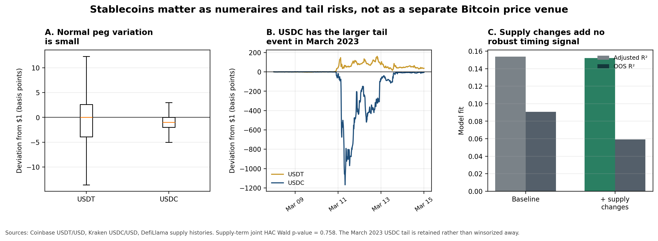
Figure 15. USDT and USDC peg behavior, the March 2023 USDC tail event, and timing-model fit with and without lagged stablecoin supply changes.
Sources: Coinbase USDT/USD, Kraken USDC/USD and DefiLlama stablecoin supply histories. The supply-term joint test uses HAC inference.

11. A practical regime map
The empirical answer depends on the regime. Before reading the table, note the distinction: trade-price timing follows executed transactions; quote-midpoint timing follows revisions to the best bid and ask; durable-price evidence comes from the long-run common-price models; persistence measures how much of an initiating move remains. The table keeps these questions separate rather than compressing them into one winner label.
Table 7. Practical regime map
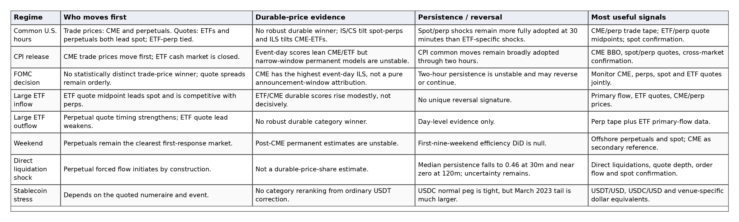
Source: SharpeEdge Capital synthesis. Durable-price evidence is concentrated in overlapping U.S. hours; direct-liquidation and depth results use sampled first-of-month data.
12. What the shifting first-response market means
For traders
The relevant tape depends on both clock and price type. CME and perpetual trade prices are the first scheduled-news references, while ETF and perpetual quote midpoints both reprice ahead of spot during U.S. hours. On weekends, perpetuals remain the clearest timing market. Spot remains an important confirmation layer because spot-originating shocks are highly persistent in the overlapping window.
For execution desks
Timing is not execution quality. Median quoted spreads in the derived full-sample summaries are roughly 0.0015 basis points on the selected spot venues, 0.015 basis points on the selected perpetuals, 2.53 basis points for the ETF category and 5.14 basis points for CME. Top-of-book quoted notional is largest for CME and the perpetuals, while sampled Tardis depth also favors the perpetual books. Those figures do not include fees, complete depth, slippage or recovery after a market order, so they support relative capacity comparisons rather than a universal cheapest-venue ranking.
For allocators
Primary flows and secondary ETF turnover must remain separate. ETF quote midpoints move quickly on large inflow days, yet high-volume/low-flow days can show equally strong ETF timing, and large outflows shift the quote-timing balance toward perpetuals. Allocation monitoring should combine creations/redemptions with ETF quotes, CME and perpetual prices.
For risk managers
Direct forced-flow evidence now supports - but does not conclusively prove - a reversal channel. Liquidation-originating moves are much less adopted at 30 and 120 minutes than matched shocks, and the two-hour continuation difference is economically large. Margin and basis-risk systems should model the initiating flow, cross-venue transmission and subsequent adoption separately.
For regulators
Bitcoin has several connected institutional centers: offshore perpetual leverage, regulated CME derivatives and U.S. ETFs. Quote and depth evidence shows that connection quality depends on active liquidity, not merely reported volume. The policy question is whether arbitrage, collateral, surveillance and operational resilience keep cross-market price transmission orderly across jurisdictions and around forced-flow events.
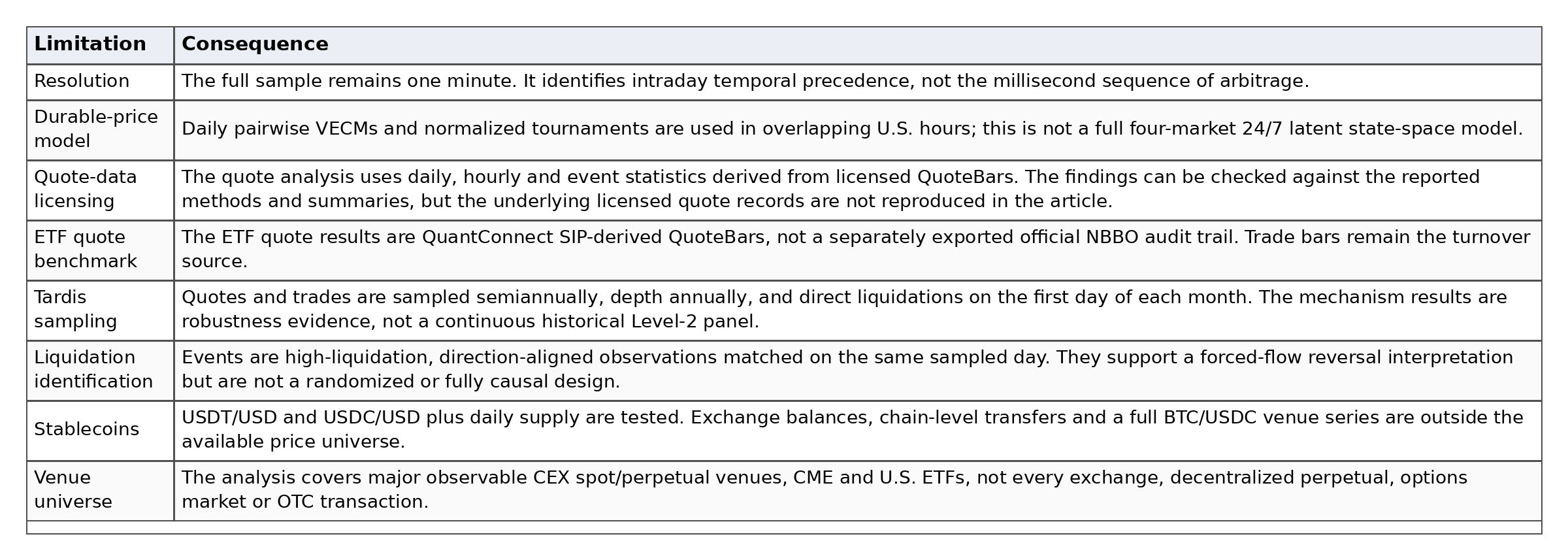
13. Limitations
Table 8. Remaining boundaries on interpretation
14. Conclusion
Bitcoin does not have one permanent home market. It has a network of prices serving different clocks, investor groups and balance-sheet constraints.
Perpetuals process 68.0% of selected-venue turnover in the common U.S. window, yet receive only about one quarter of every normalized durable-price score. IS and CS tilt toward spot and perpetuals; ILS tilts toward CME and ETFs; a five-fund return composite removes the ETF edge. The durable price remains shared and the ordinal ranking remains fragile.
Which market moves first depends on the price measure and the regime. CME and perpetual trade prices move first during many U.S. hours, while ETF and perpetual quote midpoints both lead spot and are statistically tied with each other. Trade prices record executions and quote midpoints record revisions to the best bid and ask, so the two results are complementary rather than competing. Market structure - active quotes, top-book capacity, imbalance and volatility - explains daily timing variation far better than turnover alone.
The direct-liquidation test provides a focused stress result. Across 67 matched pairs, liquidation shocks are progressively less adopted and lean toward reversal by two hours. The economic difference is large, but the rank-based p-value remains above 0.05, so the result is suggestive rather than conclusive. Stablecoin evidence is similarly nuanced: USDC is tighter in normal conditions but has a much larger depeg tail, while daily USDT and USDC supply changes add no robust timing signal.
These findings reconcile rather than erase the literature disagreements. Different products, frequencies and estimators answer different questions. Bitcoin increasingly resembles a market with several connected centers of price formation: the first-moving market rotates, durable attribution is shared, and liquidity influences how prices are transmitted across venues.

Technical appendix
This appendix documents the implementation, equations, data-quality rules, robustness checks and data sources used in the analysis. Source files were checked for completeness, timestamp consistency and internal integrity before estimation. Licensed quote data enter through derived daily, hourly and event statistics rather than raw record reproduction.
A. Data sources and quality
Table A1. Core data inventory
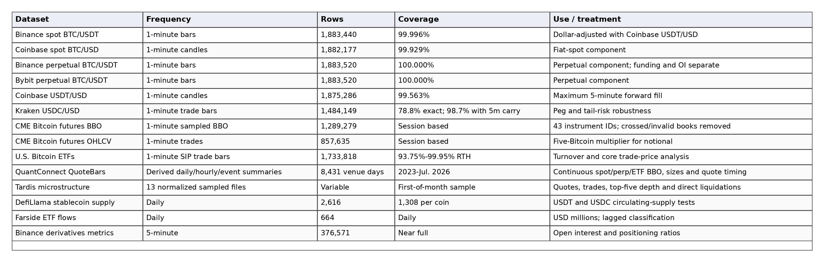
Sources: Binance and Bybit archives/APIs; Coinbase; Kraken; Databento; Alpaca SIP; QuantConnect derived QuoteBars; Tardis; DefiLlama; Farside.
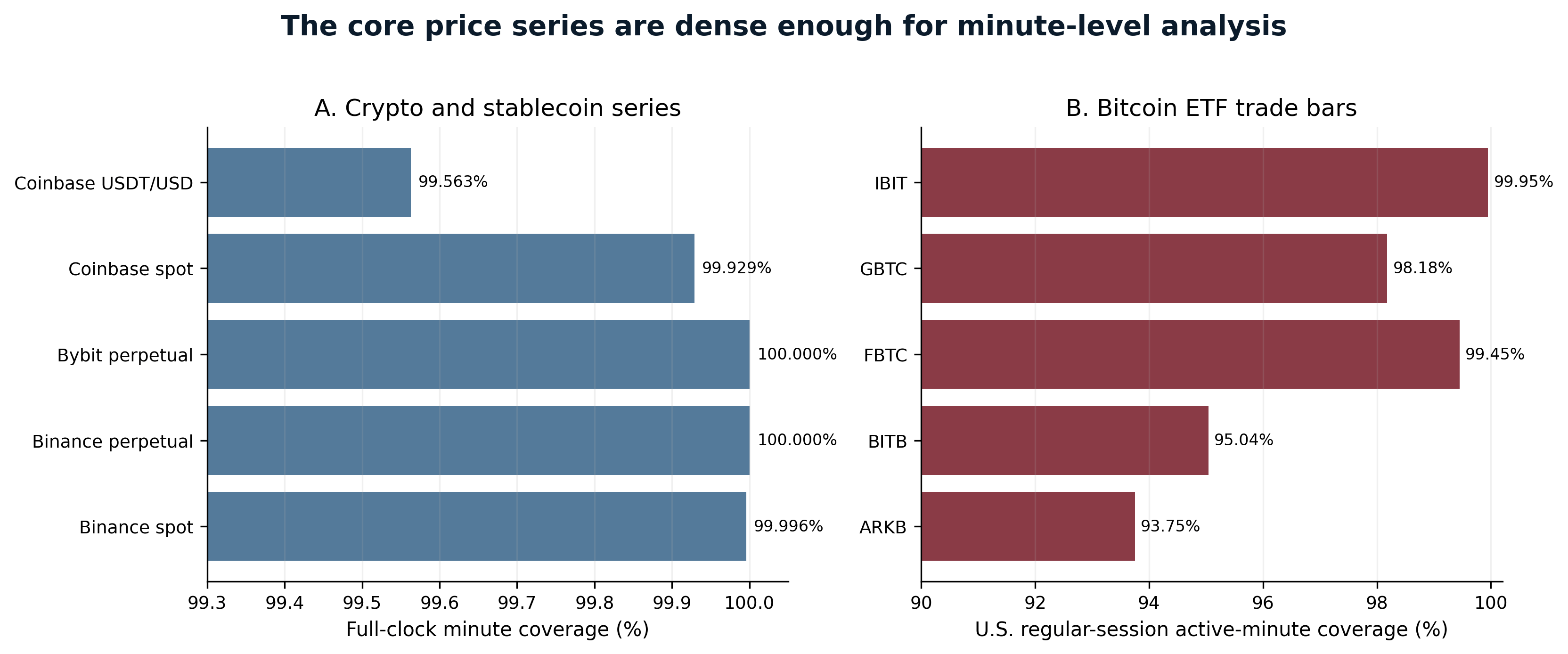
Figure A1. Full-clock coverage of crypto and stablecoin series, and active-minute coverage of ETF regular-session trade bars.
Source: SharpeEdge Capital data-quality audit.
CME BBO quality is high after cleaning. Of 1,289,279 records, 1,030 are crossed, 81 locked and 44 have nonpositive or missing quote or size values. Locked quotes are retained for midpoint calculations but excluded from positive-spread summaries. The median quoted spread is 5.14 basis points; the 95th and 99th percentiles are 9.79 and 13.84 basis points. For BBO-1m, the interval timestamp is ts_recv minus one minute; an undefined last-trade timestamp does not invalidate an otherwise usable quote.
B. Method provenance, formulas and symbol guide
Table A2. Which methods are standard and which implementation choices are specific to this study
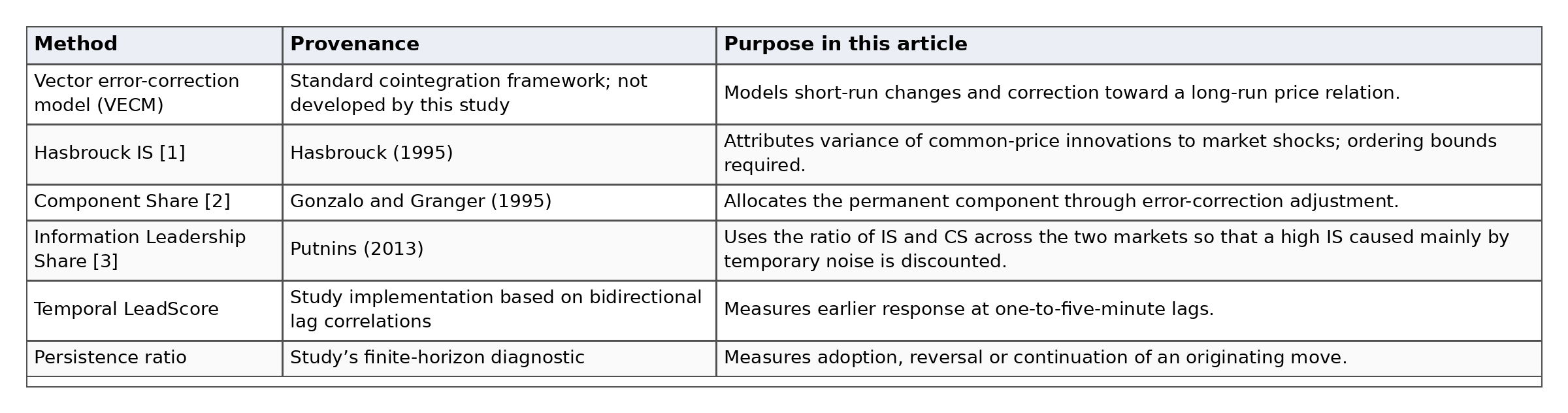
Table A3. Formula and symbol guide
C. Category construction
The spot and perpetual category prices are geometric means: equal-weight averages of log prices. Both USDT-quoted components are converted to dollars before aggregation. Category returns are exact one-minute log differences; no long forward fill is used.


Table A4. Arithmetic-versus-geometric mean diagnostic

CME uses the BBO midpoint and removes returns on instrument-ID transition minutes. ETF timing uses IBIT because regular-session active-minute coverage is 99.95%. The category robustness composite uses the median available return across IBIT, FBTC, GBTC, ARKB and BITB; it does not average incomparable share-price levels.
D. Daily pairwise common-price model
For each trading day and category pair in the 10:00-15:55 ET window, 5-minute log levels enter the fixed-beta VECM. Five-minute intervals reduce one-minute market noise while retaining intraday adjustment; log prices make proportional changes comparable across instruments with different dollar levels:

Delta p_t is the vector of 5-minute log-price changes. The expression in parentheses is the previous interval’s deviation from the day’s mean pairwise spread. alpha is the vector of error-correction speeds: it shows how strongly each price reacts when the pair diverges. Gamma captures one lag of short-run return dynamics. u_t is the vector of unexpected residual shocks. A valid day requires at least 60 observations, a mean-reverting spread and stable adjustment coefficients. The model yields IS bounds and midpoint, absolute CS, ILS, residual correlation and spread half-life.
Table A5. Method sensitivity in the common U.S. window

Table A6. Pairwise diagnostics

E. Temporal-precedence model
For pair i,j and lag k, the score is the difference between corr(r_i,t, r_j,t+k) and corr(r_j,t, r_i,t+k). Lags 1-5 receive weights proportional to 1/k. Weekly estimates are averaged, and a category’s net score is the mean signed score across available pairs. The top hour-of-week category is declared distinct only when the margin over second place exceeds 1.96 pooled standard errors, the standard pointwise 95% normal-approximation cutoff. A 1.64 cutoff colors 85 cells; a 2.58 cutoff colors 49, with only perpetuals and CME appearing as distinct winners under all three thresholds.
Table A7. Temporal-precedence scores by session
F. Persistence analysis
Large category-specific return shocks are selected independently within the relevant availability window. The common response is the cross-category median return. Selection thresholds and spacing are symmetric. The ratios are evaluated at 1, 5, 30 and 120 minutes and are not constrained to be monotonic.
Table A8. Common U.S. persistence ratios

G. Event modules
G.1 Scheduled macro events
Table A9. CPI and FOMC timing and event-day results

Table A10. CPI and FOMC common-response persistence

Table A11. Unstable narrow-window permanent-price estimates

G.2 Allocator-flow regimes
Table A12. Allocator-flow regimes

G.3 Leverage-stress proxies
Table A13. Leverage-stress proxy results

G.4 CME weekend schedule expansion
Table A14. Early CME weekend results

Table A15. Exploratory post-launch weekend permanent-price tournament

The difference-in-differences model includes hour-of-week and week fixed effects. The post x weekend coefficient is +0.139 basis points (SE 0.142, p=0.324, N=43,985).
H. Stablecoin and category robustness
Table A16. USDT numeraire correction

Table A17. Principal robustness checks

I. Continuous quote and execution-quality results
Table A18. Continuous top-of-book execution summaries
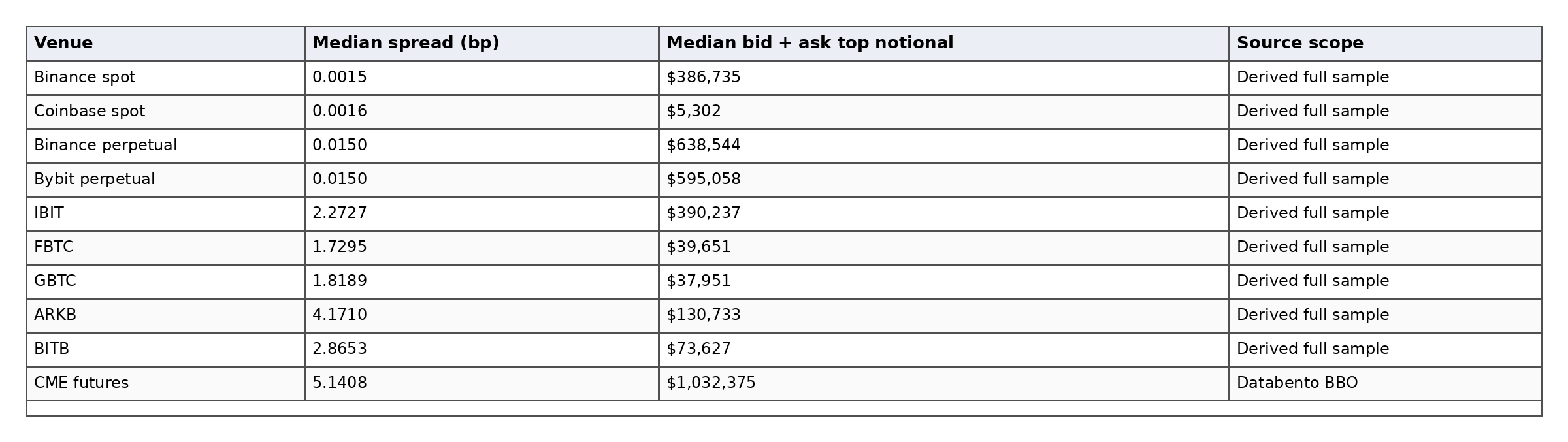
Table A19. Turnover-versus-microstructure timing models

Table A20. Combined quote-timing model coefficients

The dependent variable is the daily perpetual-over-spot quote-midpoint lead score. Predictors are winsorized, standardized and estimated with HAC standard errors. Out-of-sample R-squared uses an expanding-window ridge model. These are explanatory associations, not trader-level causal effects.
J. Sampled depth, trade size and direct liquidations
Table A21. Tardis sampled microstructure

Table A22. Direct-liquidation persistence versus matched controls

Table A23. Direct-liquidation minus control differences

K. USDT, USDC and stablecoin supply
Table A24. Stablecoin peg diagnostics

Table A25. Stablecoin-supply predictive test

References and evidence notes
1. Hasbrouck, J. (1995). One Security, Many Markets: Determining the Contributions to Price Discovery. Journal of Finance 50(4), 1175-1199.
2. Gonzalo, J., and C. Granger (1995). Estimation of Common Long-Memory Components in Cointegrated Systems. Journal of Business & Economic Statistics 13(1), 27-35.
3. Putnins, T. J. (2013). What Do Price Discovery Metrics Really Measure? Journal of Empirical Finance 23, 68-83.
4. Baur, D. G., and T. Dimpfl (2019). Price Discovery in Bitcoin Spot or Futures? Journal of Futures Markets 39(7), 803-817.
5. Gemayel, R., T. Franus, and J. Bowden (2023). Price Discovery Between Bitcoin Spot Markets and Exchange-Traded Products. Economics Letters 228, 111152.
6. Frino, A., R. Gaudiosi, R. I. Webb, and Z. I. Zhou (2025). Price Discovery in Bitcoin Spot or Futures? The Jury Is Out. Journal of Futures Markets 45(4), 269-288.
7. Mohamad, A. (2025). Do Bitcoin ETFs Lead Price Discovery Following Their Introduction in the Bitcoin Market? Computational Economics 66, 947-969.
8. Kia, K., B. Liu, Q. Li, V. Song, and K. Xu (2026). Price Discovery in Bitcoin ETF Market. Financial Review 61(2), 435-449.
9. U.S. Securities and Exchange Commission (10 January 2024). Statement on the Approval of Spot Bitcoin Exchange-Traded Products.
10. U.S. Securities and Exchange Commission (29 July 2025). SEC Permits In-Kind Creations and Redemptions for Crypto ETPs.
11. Coinbase Derivatives (9 May 2025). 24/7 Futures Trading Has Arrived.
12. CME Group (1 June 2026). CME Group Announces Launch of 24/7 Cryptocurrency Futures and Options Trading; schedule effective 29 May 2026.
13. Binance. Public historical data archive and developer documentation, including spot/futures klines and WebSocket market streams.
14. Coinbase Exchange public market-data API.
15. Bybit V5 public market-data and order-book WebSocket documentation.
16. Alpaca Market Data API documentation and subscription plans.
17. Databento historical data documentation and pricing.
18. Farside Investors. Bitcoin ETF Flow - All Data.
19. Federal Reserve Board. FOMC calendars, statements and meeting information.
20. U.S. Bureau of Labor Statistics. Consumer Price Index release calendars.
21. QuantConnect. Research Environment documentation for historical Crypto and Crypto Futures QuoteBar data.
22. Tardis.dev. Downloadable historical CSV datasets for quotes, trades, order-book snapshots and liquidations.
23. Kraken API Center. Public post-trade endpoint used to retrieve spot trade history.
24. DefiLlama. Downloadable stablecoin datasets with circulating supply, price and chain distribution.
25. Circle (12 March 2023). $3.3 Billion of USDC Reserve Risk Removed, Dollar De-peg Closes.
26. Federal Deposit Insurance Corporation (13 March 2023). FDIC Acts to Protect All Depositors of the Former Silicon Valley Bank.
Data provenance note
Completeness, timestamps, schemas and file hashes were checked before estimation. Licensed QuantConnect records were summarized inside the research environment; no raw licensed records or credentials are reproduced.
Author and use of AI note
Author note. This article was written and edited by Ismael Diamoutene, founder of SharpeEdge Capital, a quantitative investment firm specializing in digital assets and fiat currencies. The views expressed are the author’s research views and should not be interpreted as investment advice, an offer to sell securities, or a solicitation to invest.
Use of AI. AI tools were used as a research and drafting assistant to help structure the article, refine wording, check consistency, format tables and figures, and prepare the publication-ready document. The data sources, analytical framing, final interpretation, and conclusions were reviewed and selected by the author. Any errors or omissions remain the author’s responsibility.