Table of contents
Summary
1. Research question and scope
2. Quantum events versus quantum fear
3. How the study works, in plain terms
4. Event selection
5. Event-source notes
6. Data and variables
7. Results
7.1 The broader market-structure map
7.2 Increased ETF outflows around quantum-risk episodes
7.3 ETF adjudication checks
7.4 ETF trading-day windows
7.5 Re-anchor checks
7.6 Other channels remain null or inconclusive
8. Interpretation
9. Multiple-testing and small-sample caveat
10. Limitations
11. Reproducibility note
12. Conclusion
Appendix A. Data sources and variable definitions
Appendix B. Event catalog and source notes
Appendix C. Reproducibility and data-use notes
Appendix D. Quantitative and statistical methodology
Summary
On March 31, 2026, Google Quantum AI publicly discussed research indicating that breaking 256-bit elliptic-curve cryptography may require substantially fewer quantum resources than earlier estimates suggested. Although it doesn’t make cryptocurrencies unsafe today it caused a lot of reactions from market participants. There is no public evidence of a fault-tolerant quantum computer currently capable of breaking Bitcoin’s cryptography, but the possibility of it happening can have market implications.
Quantum risk has a longer history in crypto markets. For years, it lived mostly in academic cryptography, Bitcoin developer discussions, and occasional debates about exposed public keys, Satoshi-era coins, address reuse, and post-quantum migration. Those earlier discussions mattered, but they rarely became a mainstream market variable.
The visibility changed in late 2025 and early 2026 because several types of signals arrived close together: institutionally framed allocation commentary, Bitcoin-specific quantum-readiness research, the Google paper and related coverage, policy/governance discussion, and exposed-supply estimates such as Glassnode’s May 2026 work. That clustering moved the topic from abstract cryptographic tail risk toward a legitimate concern for cryptocurrency holders.
In this article, we try to answer the following question: when credible quantum-risk narratives appear, which layer of Bitcoin market structure reacts, if any?
This is a multi-channel market-structure test. It examines spot-Bitcoin ETF flows, native holder behavior, short-term- and long-term-holder SOPR (spent output profit ratio, a measure of whether moved coins are realized at a profit or loss), leverage and forced-selling proxies, daily absolute returns, available options proxies such as DVOL (Deribit’s implied-volatility index) and the IV-RV spread (implied volatility minus realized volatility), Bitcoin price-path conditions, and broad sentiment/attention proxies.
The findings are summarized below.
Key findings.
· Most market-structure channels are quiet. Holder supply, SOPR, open interest, liquidations, daily absolute returns, and most available options proxies do not show a comparable cross-episode abnormal response.
· ETF flows are the exception. Across specifications that do not include the broad sentiment-readout control, the estimated quantum-event effect on net ETF flows is roughly -$251 million to -$287 million per observed ETF trading day. After contemporaneous Crypto Fear & Greed is added, the effect remains negative but attenuates to -$140.1 million/day. The same result remains visible in the price-controlled block bootstrap (point -$251m/day; 95% CI [-$381m, -$125m]; p=0.007) and in random non-event window comparisons (p=0.010 for all random windows, p=0.006 for F&G-quartile matching, and p=0.003 for F&G-caliper matching). In simple terms, the ETF outflow around the quantum-risk windows is larger than what we usually see in comparable non-event windows.
· Quantum events and quantum fear are related but distinct. A quantum event is a specific, time-stamped information shock; quantum fear is broader attention, concern, and sentiment around Bitcoin’s quantum risk. The ETF result is primarily an event-window finding. The measured quantum fear proxies do not identify a separate, stable cross-channel quantum fear effect outside the events.
· The mechanism that causes those ETF outflows is unresolved. Quantum-risk narratives are a plausible material contributor to the ETF-flow response, but the evidence does not prove quantum-specific causality, sentiment mediation, or a broad repricing of Bitcoin market structure.
How to read the p-values. The random-date permutation compares the episode windows with thousands of non-event windows. The placebo distribution is the collection of abnormal responses from those randomly selected non-event windows. A permutation p-value is the share of placebo windows that produce a response at least as large as the observed episode response. A 5% threshold is a common descriptive convention, not proof of causality or a family-wise confirmatory test.
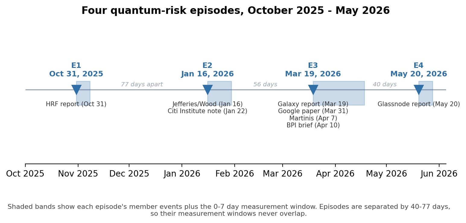
Figure 1. The four primary quantum-risk episodes on a timeline. Each episode groups events that occurred within 21 days of each other; the gaps between episodes (40–77 days) exceed the longest measurement window, so episode windows never overlap.
Two caveats belong next to the headline. First, all four primary 0–7 windows occurred during negative BTC-return windows, so ETF outflows may co-move with the broader market path rather than quantum content. Second, the strongest technical event in the catalog — the March 31 Google-paper re-anchor — does not itself show a large ETF outflow. The finding should therefore be read as a package-level, episode-window increase in ETF outflows in one market layer, not as a clean reaction to technical quantum severity.
1. Research question and scope
Bitcoin account security currently relies on ECDSA and related elliptic-curve cryptographic assumptions. A sufficiently capable quantum computer running Shor’s algorithm could in principle break the discrete-log problem underlying those assumptions. That is a real long-term cryptographic issue, but not an immediate operational one.
The market question is different. Markets can react to distant risks before those risks are technically realized. The relevant empirical question is therefore: when credible quantum-risk narratives appear, through which layer of Bitcoin market structure do they propagate?
The possible channels are distinct:
· Price path and market regime: BTC returns and BTC-return windows, used as a price-path diagnostic and control rather than as a standalone causal outcome.
· Institutional demand: spot-Bitcoin ETF net flows.
· Native holder behavior: short-term-holder and long-term-holder supply, plus SOPR.
· Leverage and forced selling: open interest and liquidations. Funding rates are acquired and verified as contextual derivatives data but are not one of the event-study outcomes in the reported tables.
· Volatility and options proxies: daily absolute returns, DVOL, IV-RV spread, options/futures OI ratio.
· General sentiment and fear: Google Trends, GDELT news proxies, and Crypto Fear & Greed.
Events are selected through documented criteria; the market response is then estimated from the data. The event categories are not meant to imply that only institutional, technical, or policy events can affect Bitcoin users. They are a screening device for this study: the goal is to isolate credible, Bitcoin-specific quantum-risk information events that are visible enough to plausibly enter market discussion. Less formal channels, social-media rumors, and non-Bitcoin quantum news may matter, but they are outside the primary event set unless they become credible, Bitcoin-specific, and market-visible.
2. Quantum events versus quantum fear
This study estimates two related but distinct effects. The first is the quantum-event effect: the reduced-form market response around screened, dated Bitcoin-specific quantum-risk episodes. The second is the quantum-fear effect: whether broader attention or concern about Bitcoin’s quantum risk moves market channels even outside the event windows.
The quantum-event test is the main event study. It asks whether ETF flows, holder behavior, leverage, forced selling, volatility, options proxies, price path, or sentiment look abnormal around the four primary episodes. The quantum-fear test is secondary. It uses observable attention and sentiment proxies — GDELT news volume/tone, Google Trends, and Crypto Fear & Greed — to ask whether a broader fear state has its own market footprint.
Do measured fear proxies peak during quantum events? The evidence is mixed. Broad crypto sentiment, measured by Crypto Fear & Greed, deteriorates after all four primary episode anchors: -5, -25, -13, and -2 points over the following seven days. Because lower Fear & Greed means more fear, that is consistent with broad fear rising during or shortly after the primary event windows.
But the pattern is not uniform across every individual event. When all eight included event dates are checked, some post-event Fear & Greed changes are flat or positive, including the Google-paper re-anchor. The event indicators also explain only a modest share of measured fear-proxy variation: about 10% of news-volume variation, 5% of news-negative-tone variation, and 14% of search variation.
The implication is important. The data do not show that quantum fear cleanly peaks on every quantum-event date, and they do not show an independent, stable fear effect across all market channels. The fear proxies are noisy diagnostics because they measure aggregate attention or broad market mood, not investors’ private reasons for trading. Search volume can rise because of media repetition, news tone can reflect general crypto stress, and Crypto Fear & Greed embeds price, volatility, momentum, and activity. These proxies are therefore useful for checking whether attention and mood moved around the events, but they cannot prove that fear caused the ETF outflows or that fear was absent when a channel was quiet.
3. How the study works, in plain terms
For each episode, the analysis asks one question per market channel: was this channel unusually different in the days right after the episode, compared with its own recent normal?
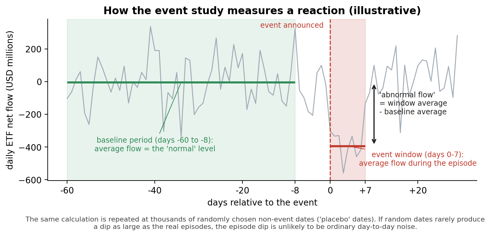
Figure 2. The core measurement, illustrated with simulated data. Each channel’s behavior in the 0–7 day window after an episode is compared with its own baseline level from the 60 days before the event (the 7 days immediately before the anchor are excluded so anticipation does not contaminate the baseline). The difference is the abnormal response. The same calculation is then repeated at thousands of random non-event dates; the share of random dates producing a response at least as large is the permutation p-value.
Three details matter for honest measurement. Slow-drifting stock variables such as holder supply and open interest are measured as cumulative abnormal change net of recent drift. Flow variables such as ETF flows and liquidations are measured as baseline-mean level deviations. Available volatility and options proxies are measured in levels or spreads, with specific caveats noted below.
Standardization puts unlike channels on a common scale. One sigma means that the response is one normal non-event standard deviation away from that channel’s own normal variation. This is useful because ETF flows, holder supply, open interest, SOPR, and volatility are measured in different units. Raw dollar or native-unit values are also reported so the reader does not have to rely only on sigma units.
The random placebo dates create the comparison distribution. A placebo window is a randomly chosen non-event window of the same length as the real episode window. The analysis repeats the same abnormal-response calculation at thousands of these non-event windows. The distribution of those placebo responses tells us whether the real episode response is unusually large relative to normal market noise.
Daily absolute return is used as the primary volatility proxy because it is non-overlapping. Shorter rolling realized-volatility windows can be tested as robustness checks, but they reuse observations from the event and nearby baseline windows, which can mechanically mix the response with the measurement window. Absolute daily return is simpler and avoids that overlap problem.
4. Event selection
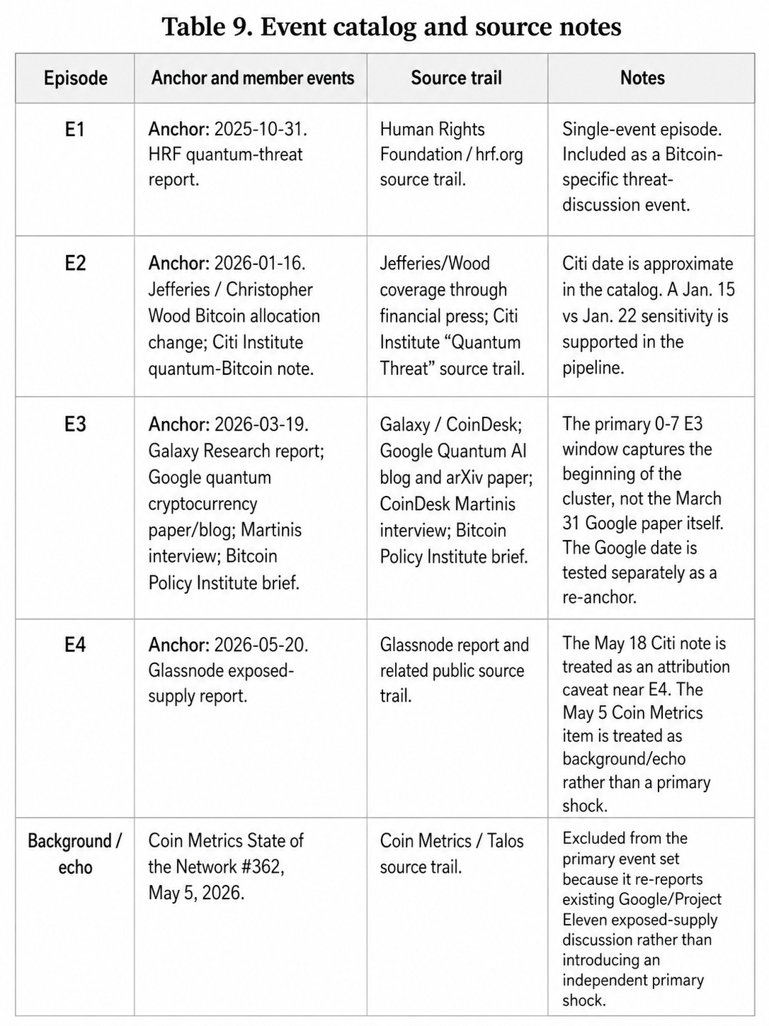
The study begins with a screened catalog of candidate Bitcoin-specific quantum-risk events between July 2025 and May 2026. The final primary analysis uses four temporally separated episodes:
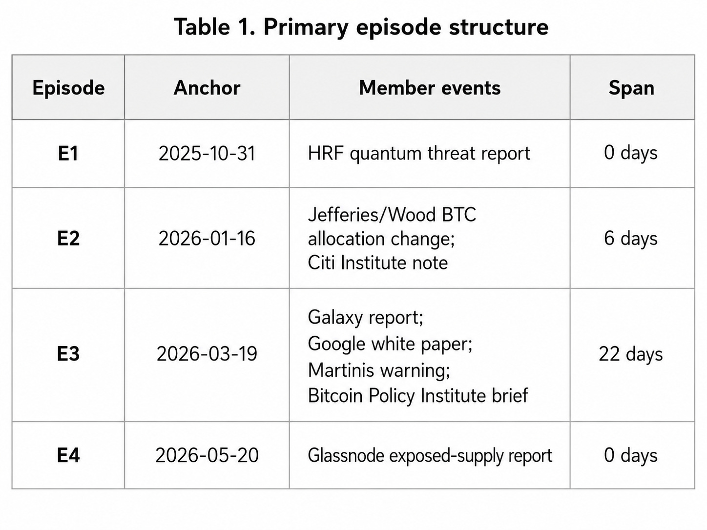
The inclusion rule is simple. An event must be Bitcoin/ECDSA-specific and credible, and the current Path A also requires novelty. That novelty gate prevents low-novelty re-reports from entering the primary event set. The Coin Metrics May 5 item is retained only as an echo/background sensitivity, not as a primary shock.
The events are clustered into episodes because several occur close together, especially in March–April 2026. Treating each as an independent 30-day shock would create overlapping windows and unstable attribution. Because the gaps between the four primary episodes exceed the longest measurement window, the episode windows do not overlap.
5. Event-source notes
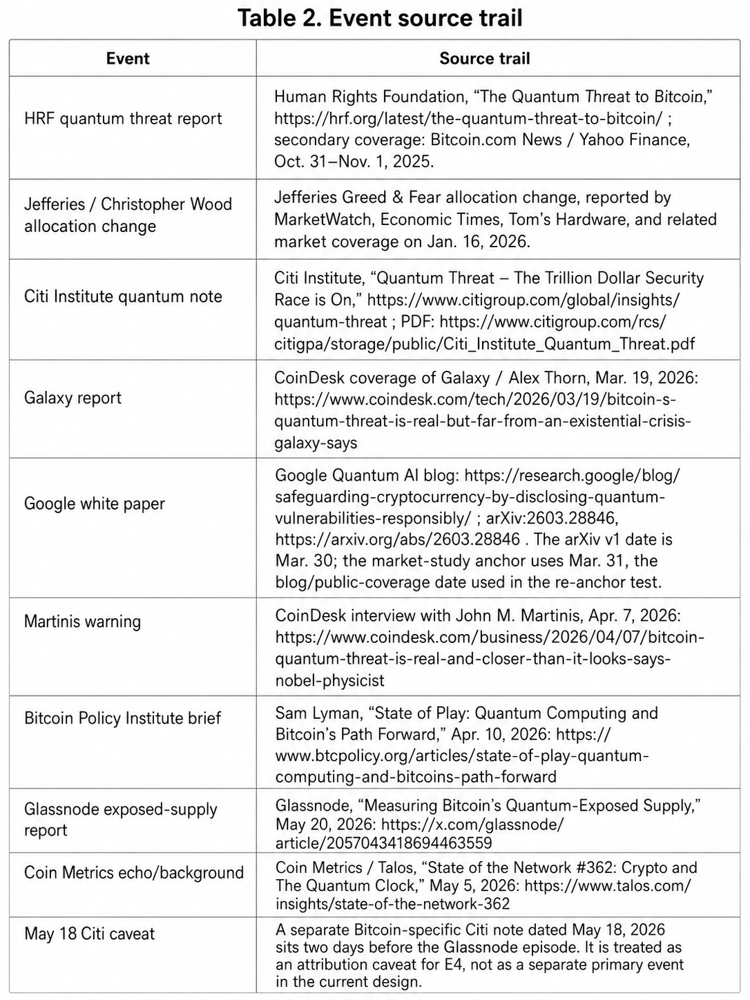
The full event-screening matrix contains all 18 candidates, their criteria scores, inclusion decisions, and source trail. The public source trail is listed here so readers can distinguish primary sources from secondary coverage.
6. Data and variables
The analysis combines price, on-chain, derivatives, ETF-flow, options, news, search, and sentiment data:
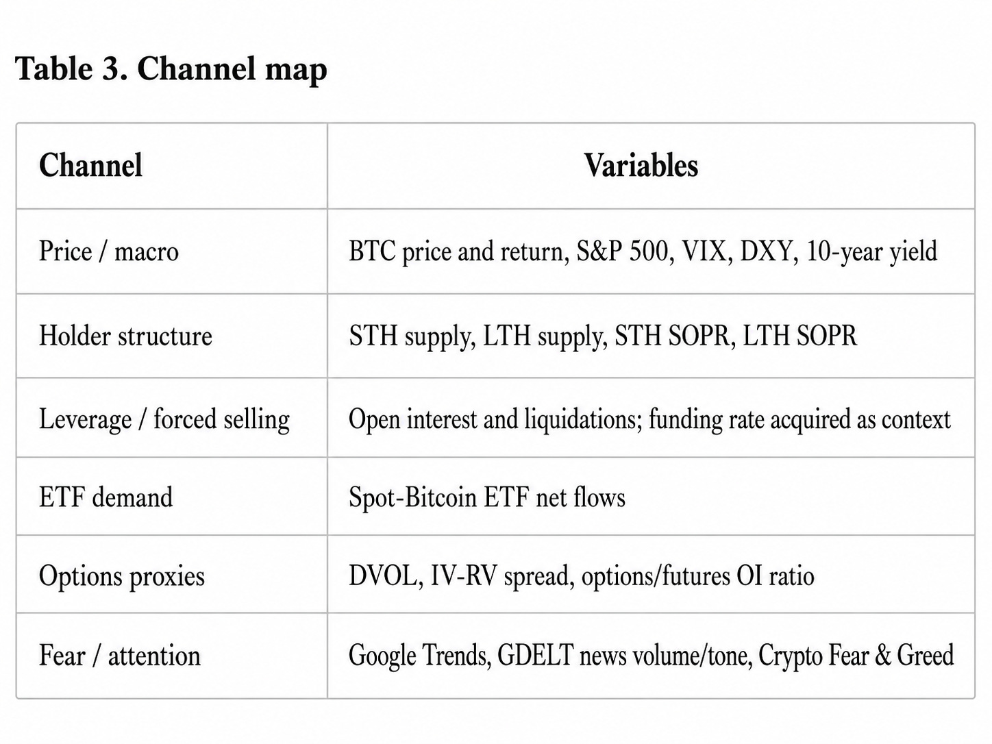
STH means short-term holder and LTH means long-term holder. SOPR means spent output profit ratio; it helps identify whether coins that move are realized at a profit or a loss. STH/LTH supply and open interest are treated as stock variables, so the main calculation adjusts for normal drift.
Coin-aging reclassification is a mechanical accounting effect: as coins remain unmoved for long enough, they can move from the short-term-holder bucket to the long-term-holder bucket even if they are not newly sold. That is why holder supply is measured as drift-adjusted cumulative change rather than as a raw level.
ETF flows are observed on trading days. Calendar event windows therefore omit non-trading days; ETF-flow magnitudes are per observed ETF trading day, not per calendar day. Because ETF flows are trading-day data and are the only channel with a persistent signal, trading-day windows are reported as a robustness check.
DVOL is Deribit’s implied-volatility index. IV-RV is the difference between implied volatility and realized volatility. IV-RV is useful but imperfect: because realized volatility is based on a rolling window, the IV-RV spread partly inherits the rolling-realized-volatility overlap issue that the main daily-absolute-return volatility proxy was designed to avoid.
7. Results
7.1 The broader market-structure map
Across the original six market-structure channels plus behavioral and options proxies, ETF flows are the only channel with a consistent negative response. This is a result of the broader market-structure test, not the starting assumption of the paper.
The episode event study shows the following average 0–7 responses in sigma units:
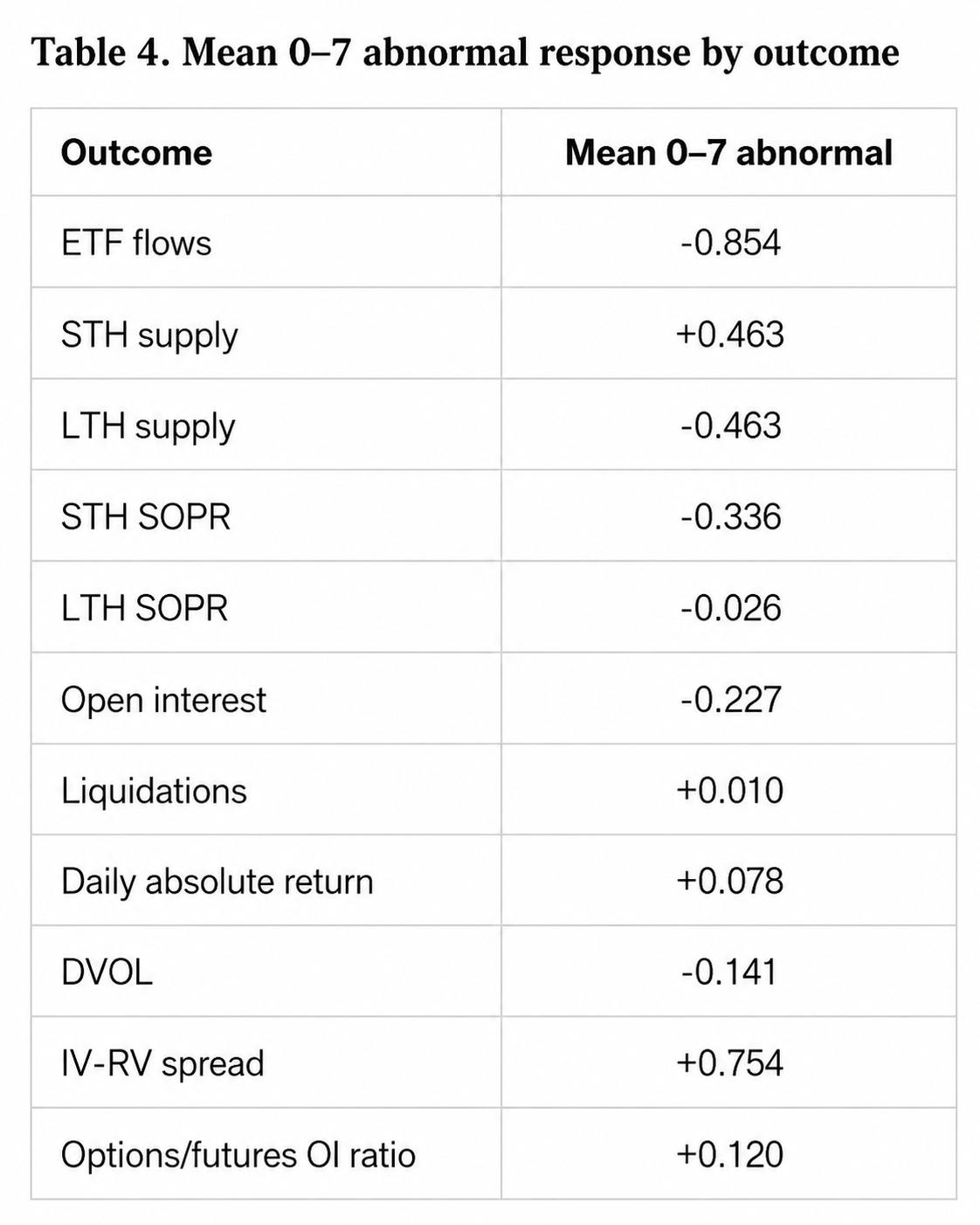
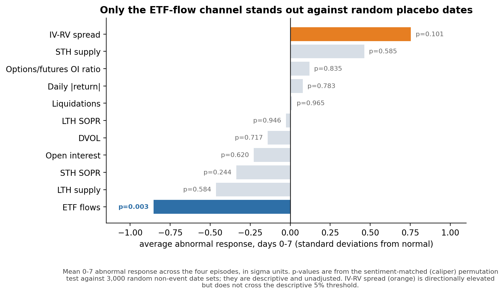
Figure 4. All eleven tested channels at once, with their sentiment-matched permutation p-values. A permutation p-value is the fraction of similar non-event windows that look at least as unusual as the real event windows. Only ETF flows fall below the conventional descriptive 5% threshold in the fine F&G-matched permutation test.
7.2 Increased ETF outflows around quantum-risk episodes
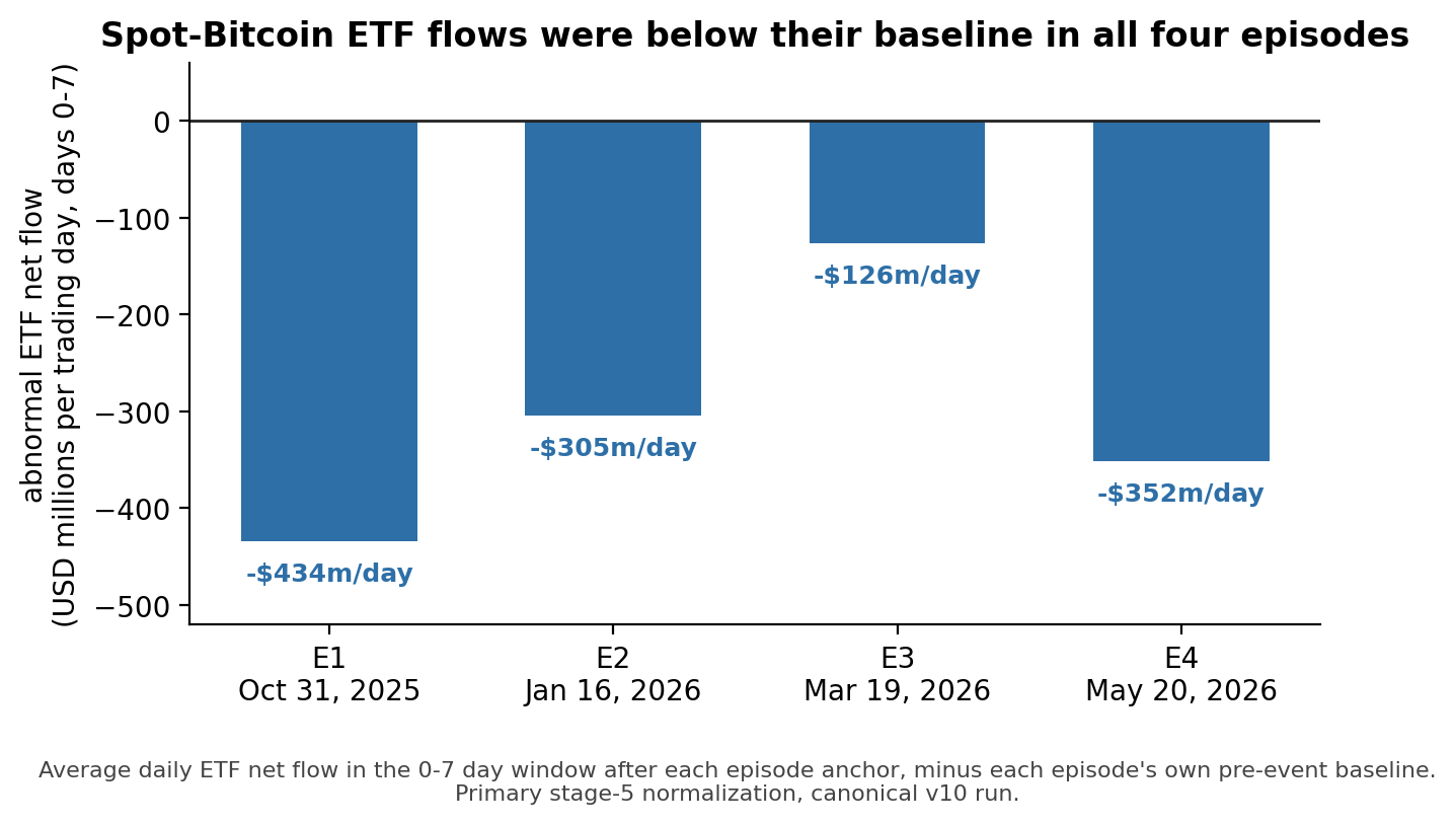
Figure 3. The headline result in dollar terms: abnormal ETF net flow per trading day over the 0–7 window after each episode, relative to each episode’s own pre-event baseline. All four episodes are negative under the primary event-study normalization.
Under the primary event-study non-event-scale normalization, the calendar-window per-episode ETF-flow abnormal is negative in all four primary episodes:
E1: -1.22 sigma; E2: -0.86 sigma; E3: -0.36 sigma; E4: -0.99 sigma.
In raw units, the 0–7 ETF abnormal responses are approximately -$434 million/day, -$305 million/day, -$126 million/day, and -$352 million/day across E1–E4. One descriptive table in the audit dossier reports E3 as slightly positive under a local-baseline trading-day heterogeneity view. That discrepancy is not caused simply by using ETF trading days. It comes from a different denominator and local-baseline choice: the primary event-study view uses event-free non-event standardization, while the heterogeneity view uses a local baseline that can be affected by earlier episode windows. The correct interpretation is that E3 is weak; the package-level ETF outflow result is not uniformly strong in every normalization.
7.3 ETF adjudication checks
The permutation statistic uses the same primary event-window normalization as the main event-study table: the observed ETF abnormal is -0.854 sigma. The permutation evidence remains exploratory and unadjusted.
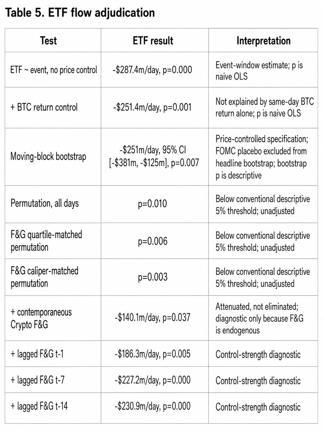
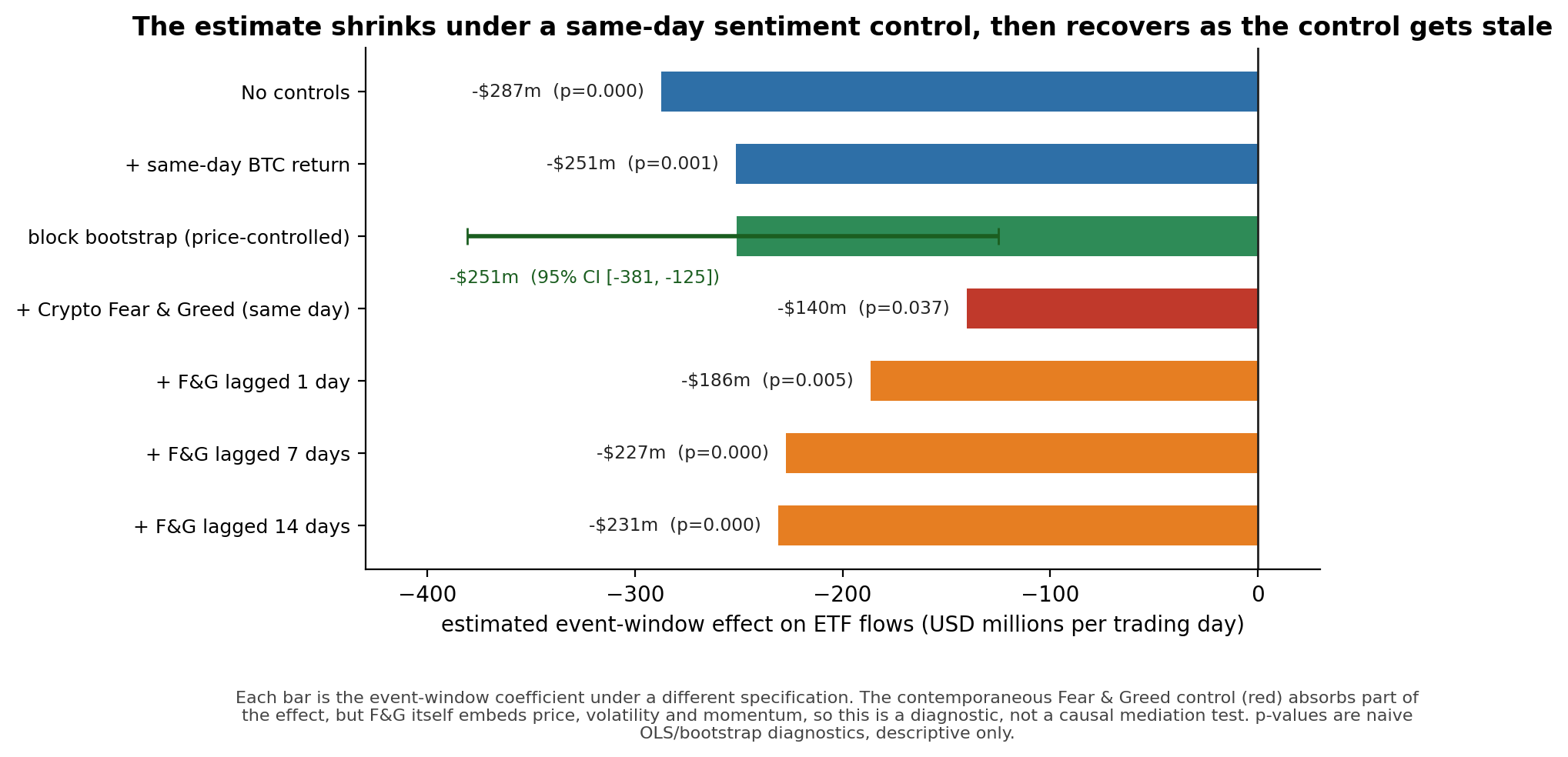
Figure 5. The ETF event-window estimate under successively stronger controls. The same-day Fear & Greed control absorbs part of the effect; lagged versions absorb less. That pattern is a control-strength gradient, not proof of mediation.
The contemporaneous F&G control materially reduces the event coefficient but does not eliminate it in the latest run. Because F&G is endogenous to the market path, borderline/non-stationary in level form over this sample, and partly built from price, volatility, momentum, and activity, this row should be read as a diagnostic, not a causal adjudication.
7.4 ETF trading-day windows
Because ETF flows are trading-day data, the analysis also computes windows using observed ETF-flow days only:
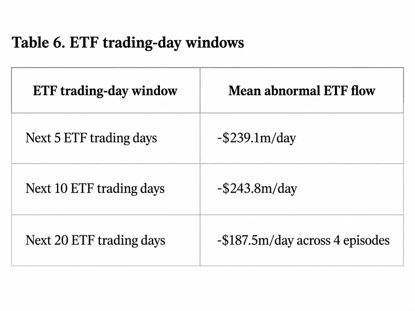
This supports the conclusion that the ETF result is not merely an artifact of calendar windows that include non-trading days. It does not mean every episode is negative under every denominator: E3 is weak and slightly positive in the local-baseline heterogeneity table. The 20-trading-day effect is smaller than the 5- and 10-day effects, which is consistent with a fading effect after the initial event window, but this pattern is not identified. It could also reflect mean reversion, other non-quantum news, or ordinary ETF-flow dynamics.
One harmonization caveat applies to this block: the trading-day windows and the descriptive heterogeneity view use local pre-anchor baselines that can be affected by earlier episode windows, while the primary event-study and permutation table use the main event-free normalization. The trading-day table is therefore a useful robustness view, not the primary estimate.
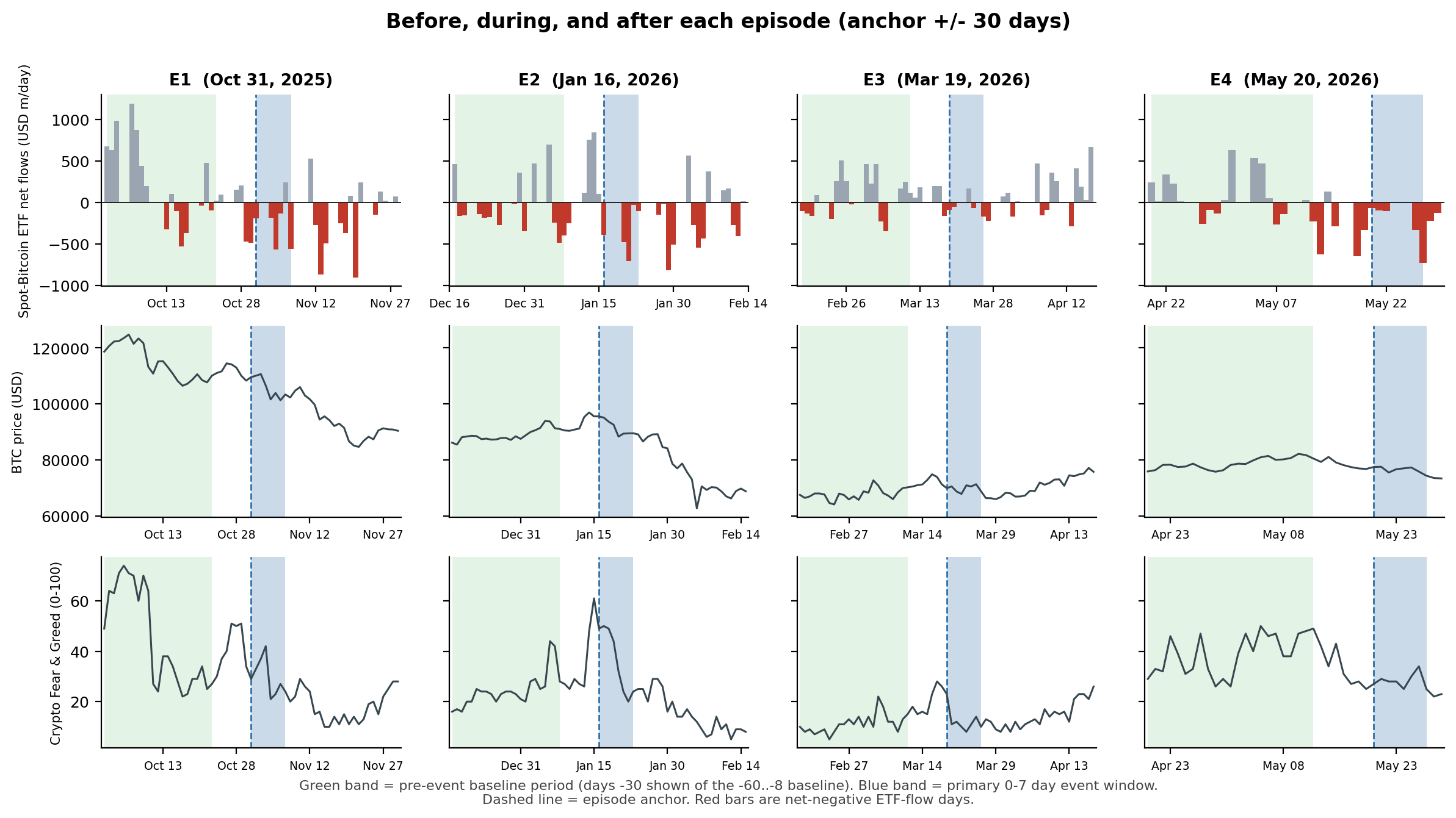
Figure 8. Before, during, and after each episode: daily ETF net flows, BTC price, and Crypto Fear & Greed from 30 days before to 30 days after each anchor. Green band = pre-event baseline period (the visible part of the 60-to-7-day baseline), red band = 0–7 day event window, gray band = 8–30 day follow-up. The figure shows why ETF-flow attribution is difficult: flows, price path, and general sentiment move together inside short windows.
7.5 Re-anchor checks
The Google paper is the strongest technical event in the catalog, but it occurs inside the broader E3 cluster. The episode design anchors E3 on March 19, before the Google paper. The study therefore includes a March 31 re-anchor check to ask whether the Google paper itself creates the same ETF-outflow pattern.
The Google re-anchor still does not show the primary ETF-outflow pattern:
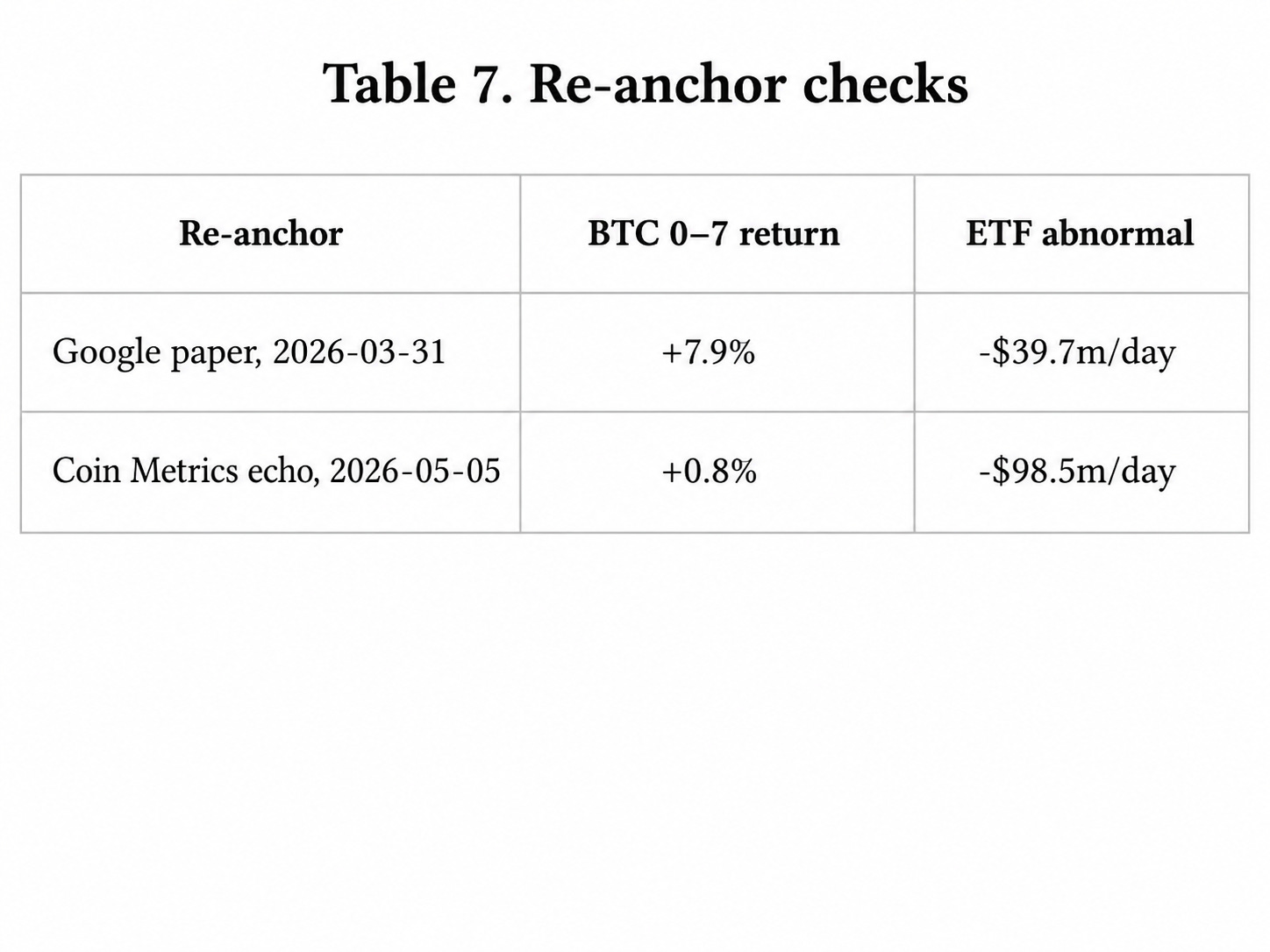
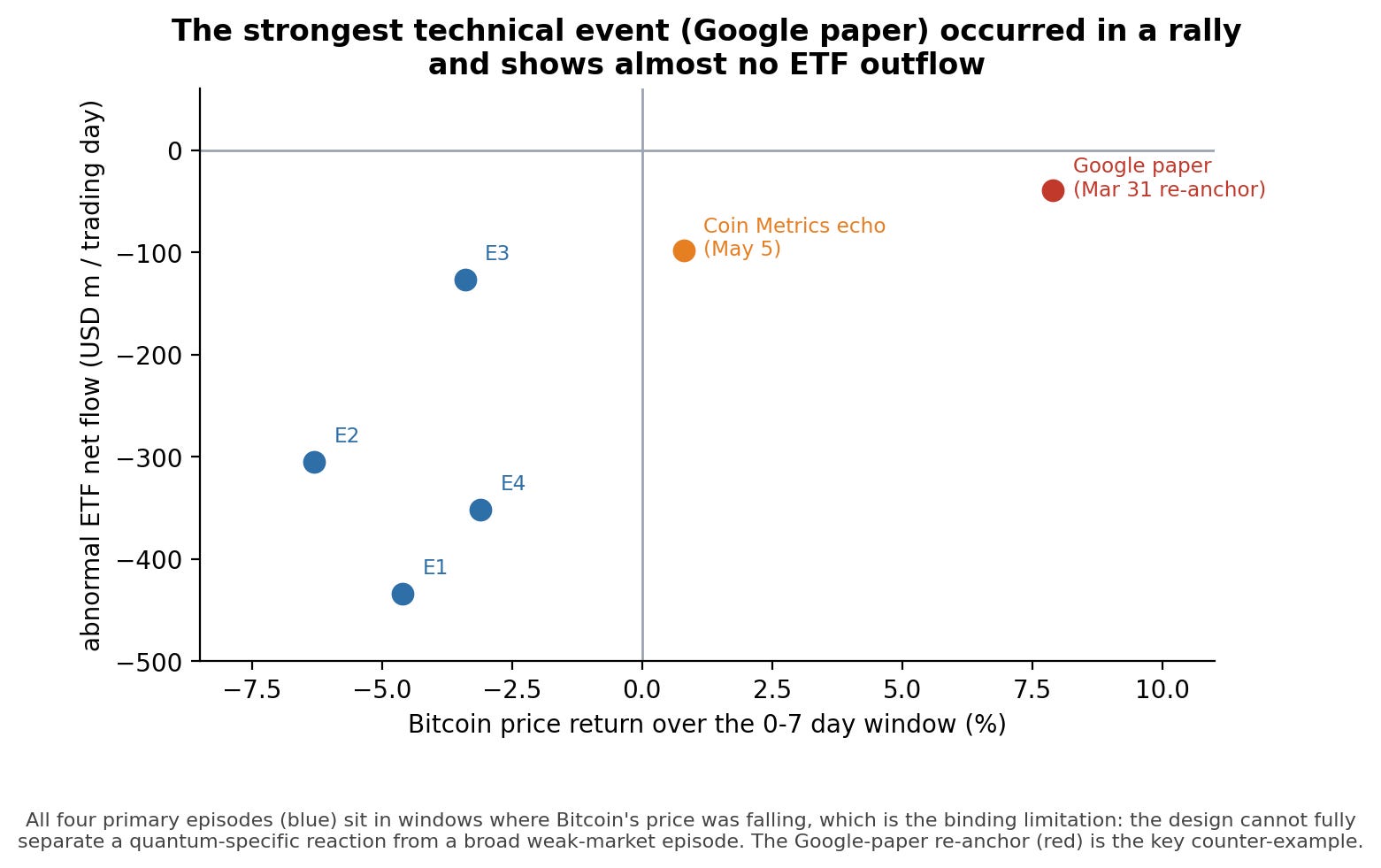
Figure 6. Why the mechanism is unidentified, in one chart. All four primary episodes (blue) sit in falling-price windows; the strongest technical event — the Google paper re-anchor (red) — occurred during a +7.9% rally and does not reproduce the ETF outflow pattern.
This is one of the main reasons the paper does not claim a clean quantum-specific mechanism. The strongest technical event occurred in a rally and does not reproduce the primary episode-window ETF pattern. That is consistent with the broader conclusion: the ETF-flow response may require a market-regime channel, an institutional packaging channel, or another coincident driver.
7.6 Other channels remain null or inconclusive
The absence of a broad market-structure response is important, but it should be read narrowly because some level variables are borderline or non-stationary in ADF checks and because available options data do not include the cleanest tail-risk measures such as historical skew or risk reversals.
The STH/LTH supply responses are mirror images, which is expected for stock measures affected by coin-aging mechanics. SOPR does not show a consistent spending response. Open interest and liquidations do not show a leverage or forced-selling response. Daily absolute returns are quiet. DVOL is quiet. IV-RV is directionally elevated, especially in E3, but it does not clear the descriptive permutation thresholds and it partly inherits the rolling realized-volatility overlap issue.
A key limitation applies to all channels: the study does not model every determinant of every channel. A large move could reflect another explanatory variable that jumped during the same window, while a small or null response could hide a quantum-related effect offset by some unrelated force. The channel results are therefore reduced-form abnormal-response tests, not structural decompositions of every market driver.
The safest statement is therefore: no other channel shows a comparably strong response under the reported permutation checks; the IV-RV spread is directionally elevated but inconclusive, and a stronger tail-risk test would require historical options skew or risk-reversal data.
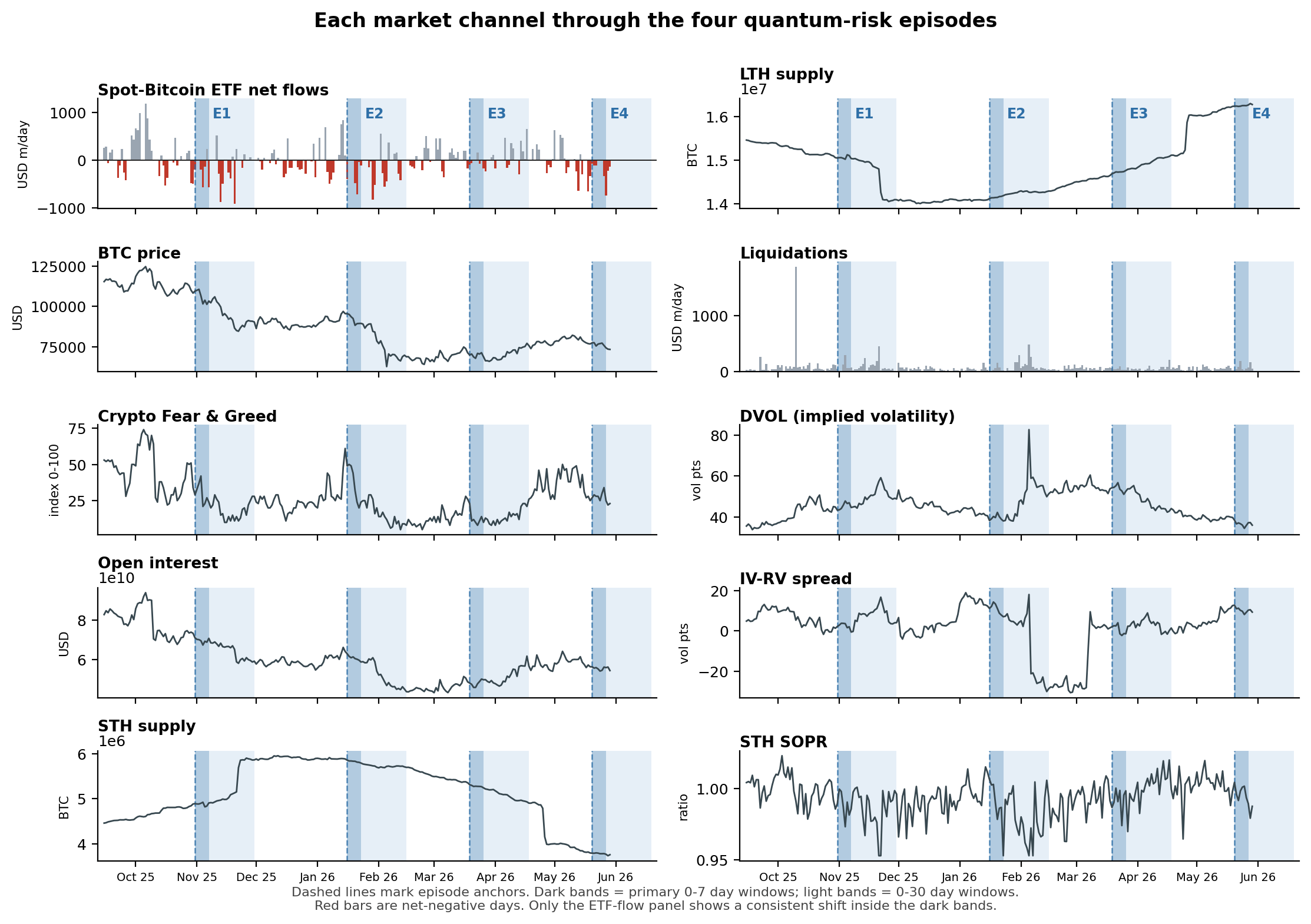
Figure 7. Every tested channel as a raw time series through the study window, with the four episode windows shaded (dark = 0–7 day primary window, light = 0–30 days). The ETF-flow panel is the only one with a visible, repeated event-window outflow pattern; other channels remain noisy or visually inconclusive.
8. Interpretation
The best current interpretation is narrow. Quantum-risk episodes are associated with a persistent increase in ETF outflows across the tested robustness checks. My reading is that quantum-risk narratives are a plausible material contributor to that response: the episodes were screened for Bitcoin-specific quantum relevance, the ETF response repeats across the primary event windows, and the response is not mirrored by broad stress in holder behavior, leverage, liquidations, volatility, or the available options proxies.
At the same time, the study has not fully modeled every determinant of ETF flows. ETF demand can be affected by portfolio-allocation cycles, macro risk appetite, basis and carry trades, issuer-specific flows, liquidity conditions, tax effects, broader risk-asset rotation, AI-related capital rotation, and general ETF-flow weakness. Because these drivers are not all structurally modeled, quantum-risk narratives should be treated as a credible candidate contributor, not as a proven root cause.
Three things are true at the same time:
· ETF flows are unusually negative around the selected quantum-risk episodes.
· Other tested market-structure channels do not respond robustly.
· The data still do not identify whether the ETF-flow response is primarily quantum-specific, quantum-fear-driven, feedback from flows into price/sentiment, or coincident with other market shocks.
The study therefore supports a bolder but still bounded interpretation: the ETF-flow response is unlikely to be dismissed as ordinary noise, and quantum-risk narratives are a credible candidate driver, but the broader Bitcoin market did not display a generalized quantum-risk repricing across the channels tested here.
That is useful. It suggests that if quantum-risk narratives currently matter for Bitcoin markets, they are most visible first through the institutional allocation layer rather than through native on-chain behavior or leverage stress.
9. Multiple-testing and small-sample caveat
The sample size is the binding constraint. The primary design has four episodes. That is enough to discipline the analysis, but not enough to establish mechanism. The ETF p-values are also vulnerable to multiple-testing concerns because the study checks many channels, windows, controls, and diagnostics.
For that reason, p-values are reported as descriptive evidence, not family-wise confirmatory inference. ETF flows are treated as the primary institutional-demand channel; the other variables are channel and falsification tests. The right next test is prospective: freeze the design and apply it to future quantum-risk events, especially events outside weak BTC-return regimes.
10. Limitations
The key limitations are:
· Only four primary episodes.
· All four primary 0–7 windows had negative BTC returns, so the design cannot separate quantum-specific repricing from a broader weak-market ETF-flow episode.
· Event clustering, especially inside E3.
· The Google re-anchor does not show the ETF-outflow pattern.
· Crypto Fear & Greed embeds price, momentum, volatility, and activity, and is borderline/non-stationary in level form over this sample, so it is not an exogenous stationary control.
· ETF flows are trading-day data while crypto trades continuously.
· Google Trends, GDELT, and other fear proxies are noisy and rate-limited; exact replication requires retaining the same cache state and data-access timestamps.
· CoinGlass licensing must be resolved before redistributing raw or derived paid-data files.
· Options-market evidence is incomplete without historical skew/risk-reversal, and the IV-RV spread is directionally elevated but inconclusive.
· The result emerged through iterative robustness work and should be frozen for future tests.
· E4 0–14 and 0–30 horizons are truncated by the sample end date (2026-05-30), so the 0–7 window and trading-day checks are the cleaner reported horizons.
· Two quantum-adjacent items sit close to E4 and remain attribution caveats for that episode: a May 18, 2026 Citi Bitcoin-quantum note and a May 21, 2026 US government $2B quantum-investment announcement that was screened out of the primary event set.
· The Citi Institute report has an official Citi page date of January 15, 2026, while the canonical event catalog keeps January 22 as a market-coverage/date-discovery placeholder. A January 15 sensitivity remains a useful robustness check.
11. Reproducibility note
Exact numerical replication requires the same data-provider access and the same frozen data snapshot. Some series require paid CoinGlass access, while GDELT, Google Trends, Deribit, and other public APIs can be rate-limited or revised. Raw CoinGlass-derived data should not be redistributed until licensing is confirmed. The code path is reproducible; exact numerical reproduction requires provider access or private frozen CSVs.
12. Conclusion
Across four credible Bitcoin-specific quantum-risk episodes, the broader Bitcoin market-structure map is mostly quiet, while spot-Bitcoin ETF flows show persistent increased outflows across the reported checks. The result is narrow, but it is not trivial.
The mechanism is unresolved. The evidence cannot distinguish quantum-specific repricing, quantum-fear-driven ETF flows, ETF-led price/sentiment feedback, or coincident within-window shocks. The most defensible claim is that quantum-risk episodes are associated with unusual institutional ETF outflows, while the rest of the tested Bitcoin market structure does not show a comparable response.
Appendix A. Data sources and variable definitions
This appendix summarizes the data sources used in the article. It is included so the reader can see what each series is meant to measure, how it enters the analysis, and which caveats apply. Raw paid-provider data are not redistributed in the public release; exact numerical reproduction requires provider access or the private frozen data cache used for the canonical run.
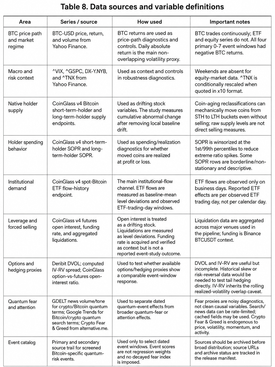
The table above is source-focused rather than result-focused. The main text reports the findings; this appendix documents what each input is intended to capture and why several channels are interpreted cautiously.
Appendix B. Event catalog and source notes
The table below summarizes the four primary episodes and the most important source trail. Events were screened for Bitcoin/ECDSA relevance, source credibility, novelty, severity, and market visibility. Closely spaced events were clustered into episodes so the main measurement windows do not overlap.
Appendix C. Reproducibility and data-use notes
· The public article is designed to be readable on its own. The technical audit dossier and replication bundle provide the full pipeline, run log, manifests, and checksum files.
· Exact numerical replication requires the same data-provider access and the same frozen data snapshot. CoinGlass-derived raw/cached CSVs are not redistributed in the public package unless licensing is separately cleared.
· If live APIs are rerun later, some Google Trends, GDELT, ETF-flow, and options-proxy values may drift because provider data and rate limits can change.
· The source manifest should be treated as the release source trail. Rows marked pending external archive should be archived before broad public distribution.
· The study is descriptive anomaly detection, not causal identification. The appendices document inputs and source trails; they do not remove the small-sample and regime-collinearity limitations discussed in the article. Appendix D gives the quantitative/statistical details behind those descriptive checks.
Appendix D. Quantitative and statistical methodology
This appendix explains the main quantitative steps behind the article. It is written for readers who want more detail than the public narrative, but less implementation detail than the full replication code.
D.1 Unit of observation and event windows
The analysis uses daily observations from January 1, 2025 to May 30, 2026. The primary event-study window is 0–7 calendar days after each episode anchor. The article also reports 0–14 and 0–30 windows in the technical outputs, but the 0–7 window is emphasized because all four episodes have complete data over that horizon and E4 is truncated for longer windows by the sample end date.
Candidate events are screened for Bitcoin/ECDSA relevance, source credibility, novelty, severity, and market visibility. Closely spaced included events are clustered into episodes using a 21-day single-linkage rule. The four primary episodes are separated by 40–77 days, so their 30-day windows do not overlap.
D.2 Baseline and abnormal-response calculation
For each channel and each episode, the event-window response is compared with a recent pre-event baseline. The baseline is the window from 60 days before the anchor to 7 days before the anchor. The 7 days immediately before the anchor are excluded to reduce contamination from anticipation or pre-event drift. Event-window days from prior episodes are excluded when constructing the primary baseline and permutation calculations.
Flow variables, such as ETF net flows and liquidations, are measured as baseline-mean level deviations: the event-window average minus the baseline average. For ETF flows, the unit is millions of dollars per observed ETF trading day because ETF flows are only observed on ETF trading days.
Stock variables, such as holder supply and open interest, are measured as cumulative abnormal change. First, the baseline daily drift is estimated from recent pre-event daily changes. Then the event-window level change is compared with the change that would be expected if the baseline drift had simply continued. This avoids interpreting normal coin-aging or open-interest drift as an event response.
For stock variables, the simplified formula is: abnormal change = (level at end of window - level at anchor) - (baseline daily drift x number of days). This is then standardized by the relevant event-free standard deviation and the square root of the window length.
D.3 Standardization and raw units
Standardization converts unlike variables into comparable sigma units. A one-sigma response means the event-window response is one normal event-free standard deviation away from that channel’s usual variation. The scale is estimated from non-event periods rather than from the event window, so a volatility spike during the event does not inflate the denominator.
Raw units are reported alongside sigma units whenever possible. This is especially important for ETF flows, where the economically meaningful number is dollars per observed ETF trading day, not only a standardized abnormal response.
D.4 Permutation tests and placebo windows
The permutation test asks whether the observed response around the real quantum-risk episodes is unusually large relative to randomly selected non-event windows. Each placebo draw selects four non-overlapping placebo anchors, mirroring the four-episode design. Placebo windows are excluded if they overlap real event windows.
The placebo distribution is the collection of abnormal responses from thousands of these random four-window draws. The permutation p-value is the share of placebo draws whose absolute average abnormal response is at least as large as the observed average response. This is an empirical random-window comparison, not proof of causality.
The article reports three permutation comparisons: all random windows, Crypto Fear & Greed quartile-matched windows, and fine Crypto Fear & Greed caliper-matched windows. The sentiment-matched versions ask whether the ETF-flow result remains unusual when the placebo windows have a similar broad crypto-sentiment level.
D.5 Bootstrap inference for ETF flows
ETF-flow observations are serially dependent: a large inflow or outflow can be followed by related flows in nearby days. A simple daily OLS standard error treats those days as too independent. The moving-block bootstrap partially addresses this by resampling contiguous blocks of daily observations rather than individual days.
The headline bootstrap is applied to the price-controlled ETF-flow specification: ETF flow = alpha + beta x quantum-event window + gamma x BTC return + error. The FOMC placebo dummy is not included in the headline bootstrap because some FOMC placebo windows overlap the quantum-event windows. The bootstrap p-value is descriptive and should be read together with the permutation tests.
D.6 Fear proxies and sentiment controls
The fear analysis uses observable proxies for attention and sentiment: GDELT news volume/tone, Google Trends search terms, and Crypto Fear & Greed. These proxies are standardized and used as diagnostics. Borderline or non-stationary proxies are retained in level-z form for comparability, so their coefficients should not be interpreted as clean stationary-control regressions.
Crypto Fear & Greed is especially important but also especially limited. It is a broad market-readout index built from price, volatility, momentum, and activity. When it attenuates the ETF coefficient, that tells us the ETF anomaly co-moves with the broader market path; it does not establish whether sentiment caused ETF flows, ETF flows affected sentiment, or both reflected another shock.
D.7 Re-anchor and echo sensitivity checks
The March 31 Google-paper re-anchor tests the strongest technical event separately from the broader March–April episode. The Coin Metrics May 5 echo check tests whether a low-novelty re-report would change the interpretation if treated as an event. These checks help diagnose whether the result is driven by technical quantum severity, by financial framing, or by broader market context.
D.8 Multiple testing and interpretation
The study examines many channels and several robustness checks. The p-values are therefore descriptive and unadjusted for the full family of possible tests. ETF flows are treated as the primary institutional-demand channel, while the other variables function as market-structure and falsification channels. The correct interpretation is anomaly detection, not causal proof.
The design can identify where abnormal responses appear in a disciplined event-study framework. It cannot fully identify why those responses occurred, because every channel has other determinants and because the four primary episodes all occurred during weak BTC-return windows.
Author and AI Use Note
Author note. This article was written and edited by Ismael Diamoutene, founder of SharpeEdge Capital, a quantitative investment firm specializing in digital assets and fiat currencies. The views expressed are the author’s research views and should not be interpreted as investment advice, an offer to sell securities, or a solicitation to invest.
Use of AI. AI tools were used as a research and drafting assistant to help structure the article, refine wording, check consistency, format tables and figures, and prepare the publication-ready document. The data sources, analytical framing, final interpretation, and conclusions were reviewed and selected by the author. Any errors or omissions remain the author’s responsibility.