When USD/JPY breached the ¥160-per-dollar mark in late April 2026, Bank of Japan current-account data suggested that Japanese authorities may have spent as much as ¥5.48 trillion in yen-buying intervention. Subsequent BOJ money-market data suggested that additional yen-buying operations may have occurred during Japan’s early-May holidays, potentially exceeding ¥8 trillion in total (including unconfirmed early-May operations). The Japanese Yen has been depreciating against the USD since mid 2025, which ultimately led to the intervention. In this article, we try to understand the historical drivers of the USD/JPY exchange rate and hypothesize on what might happen next.
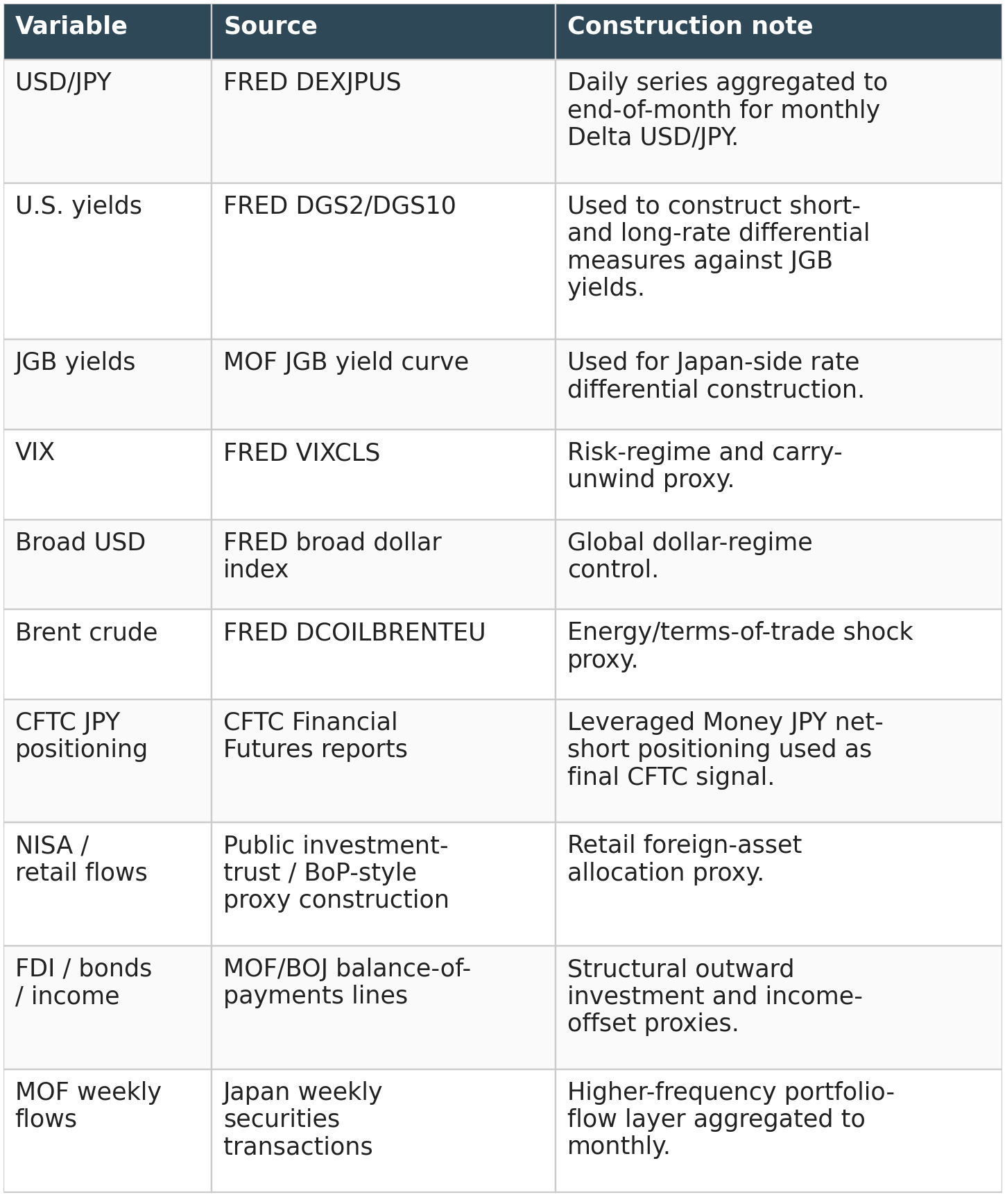
We start from available public variables that could have a causal relationship with the USD/JPY - U.S. and Japanese yields, VIX, Brent crude, broad dollar measures, CFTC positioning, Japan balance-of-payments proxies, MOF weekly securities-flow data,…. We then build a final attribution framework, translates the empirical hierarchy into a conditional probability matrix, and maps that matrix into forecast paths with explicit intervention effects.
Our analysis points to the following conclusion: monthly USD/JPY is primarily a macro-rate and dollar-regime trade, while other variables effects are mostly insignificant.
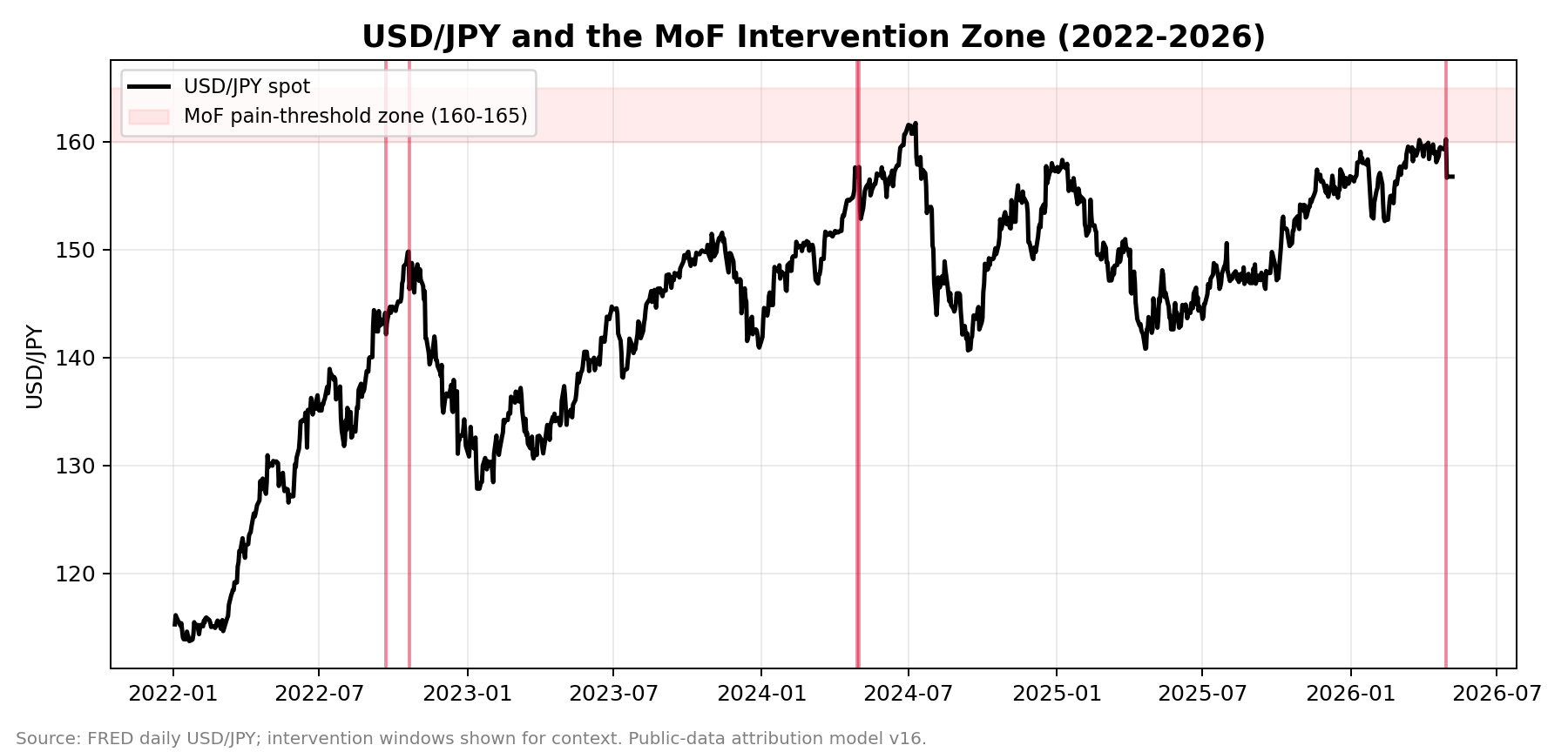
Figure 1. USD/JPY and the intervention-zone context. The red band marks the 160-165 area where intervention risk becomes a material friction rather than a structural driver.
Part I - Research Design and Final Model Architecture
The analysis separates three questions. First, what explains monthly USD/JPY variation? Second, which variables lead or transmit shocks through the system? Third, how should the empirical hierarchy be translated into a forward-looking scenario matrix? The article body focuses only on the final model stack used to answer those questions. Alternative specifications and robustness checks are placed in the appendix.
Data universe and sign convention
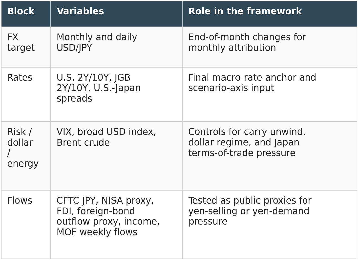
All variables are transformed so that positive values represent yen-depreciation pressure where economically appropriate. This common sign convention is essential because the model combines rates, returns, flows, income offsets, and positioning proxies. Without a consistent convention, coefficient signs and attribution shares become difficult to interpret.
Final model stack
Part II - Final Monthly Attribution Model
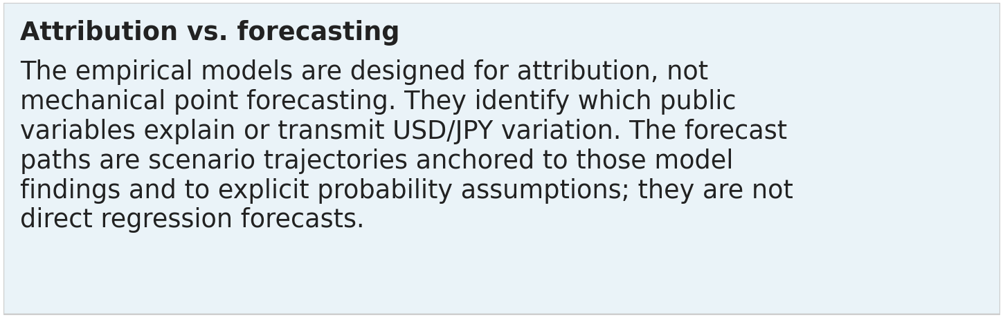
The final monthly attribution model combines macro variables and public flow proxies in a single specification. The purpose is not to declare that every coefficient is causal. The purpose is to allocate explained monthly variation across the final set of macro and flow variables after applying consistent sign conventions and robust standard errors.
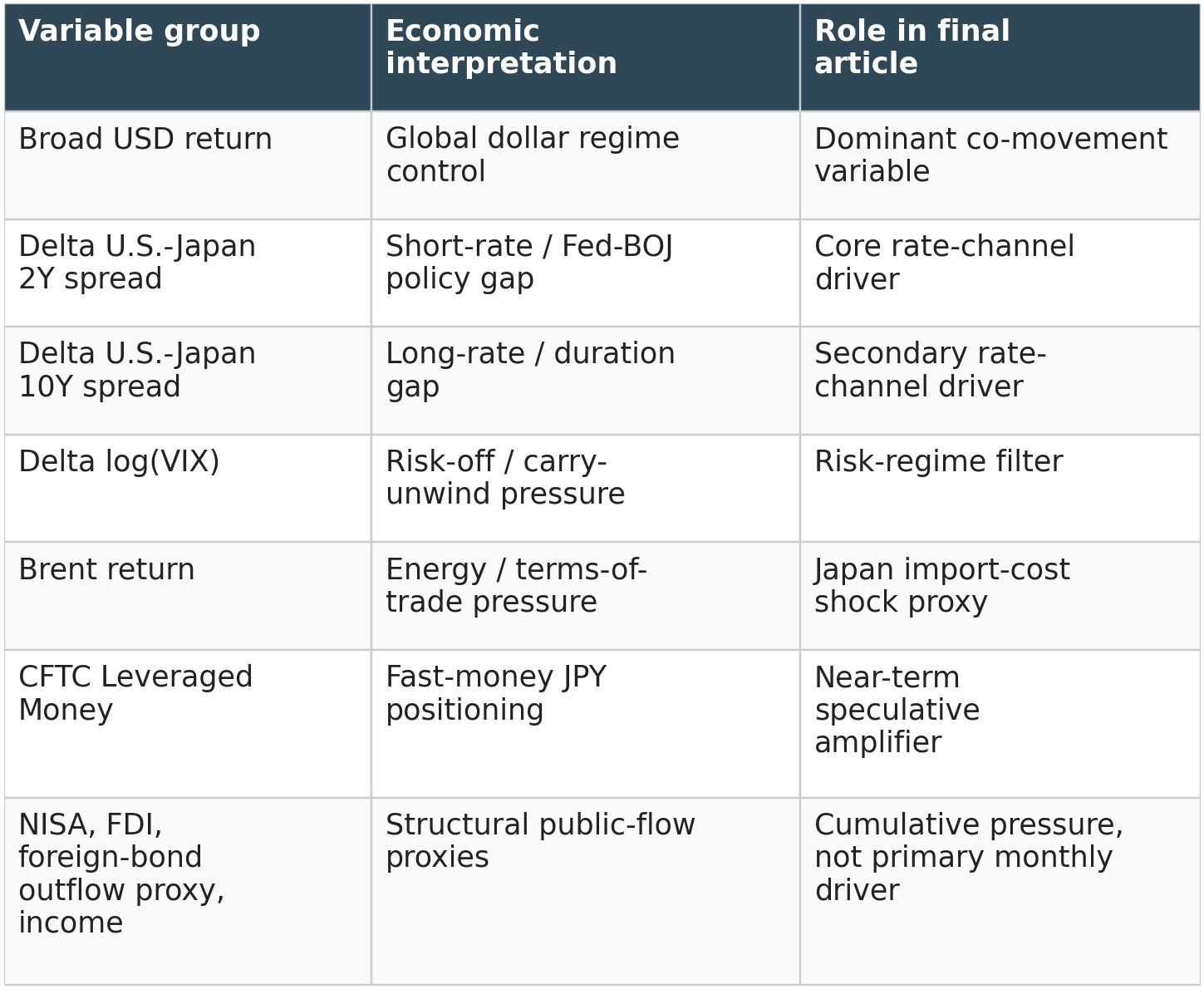
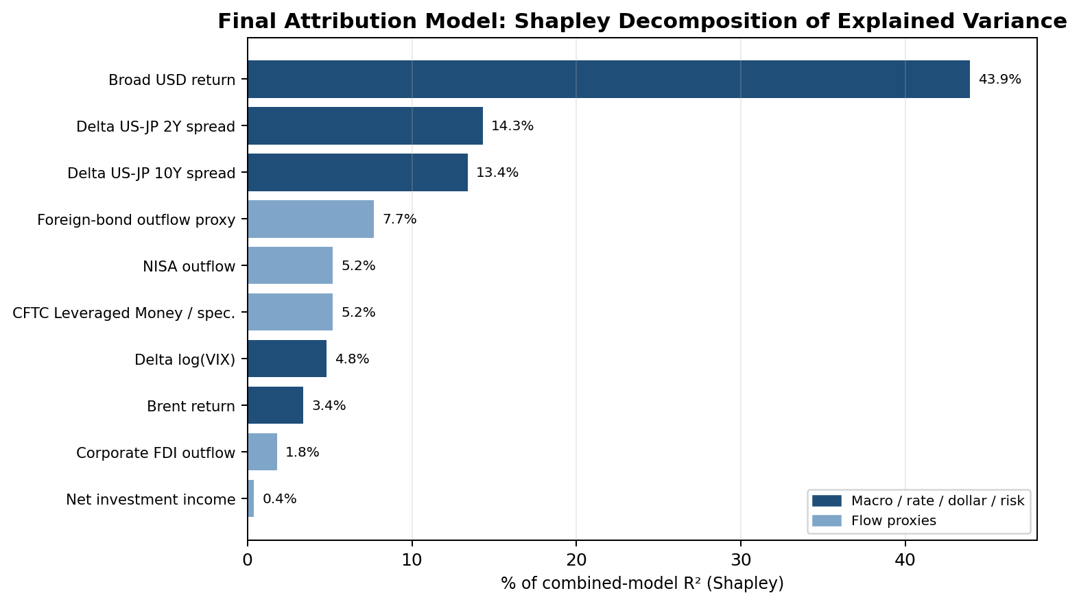
Figure 2. Final monthly Shapley attribution. Macro variables dominate the combined model; public flow proxies remain secondary and are interpreted as cumulative pressure or amplifiers.
The Shapley decomposition shows that broad USD return, the 2-year and 10-year U.S.-Japan rate spreads, VIX, and Brent account for most of the combined model fit. This does not mean that flows are irrelevant. It means that observable public flows do not carry the main explanatory burden once the macro-rate and dollar regime is included.
Directional accuracy diagnostic: The combined attribution model correctly identifies the direction of monthly USD/JPY changes in roughly 79% of in-sample months and 76% of walk-forward out-of-sample months. However, the model is best used for attribution and scenario design rather than point forecasting.
Part III - Final Dynamic Attribution: VAR and FEVD
OLS and Shapley attribution measure contemporaneous association. The dynamic attribution layer asks which variables contribute to future forecast-error variance in a system where USD/JPY, rates, risk, and flows can interact. The final VAR uses a parsimonious five-variable structure: Delta U.S.-Japan 2Y rate spread, Delta log(VIX), Delta USD/JPY, NISA outflow, and the foreign-bond outflow proxy.
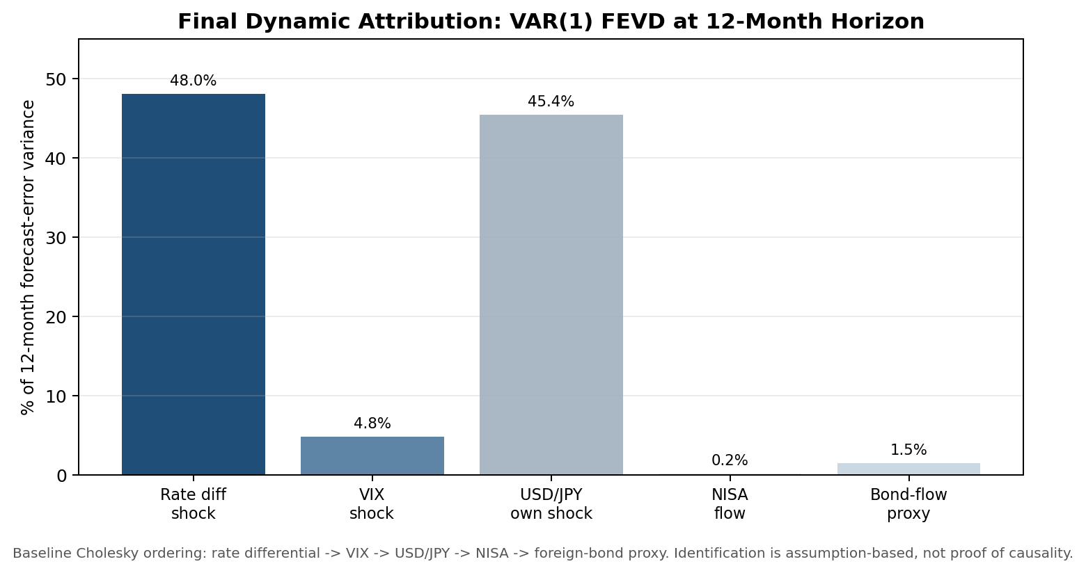
Figure 3. Final VAR forecast-error variance decomposition. The 2-year rate-differential shock is the largest identified driver; public flow shocks are much smaller under the baseline ordering.
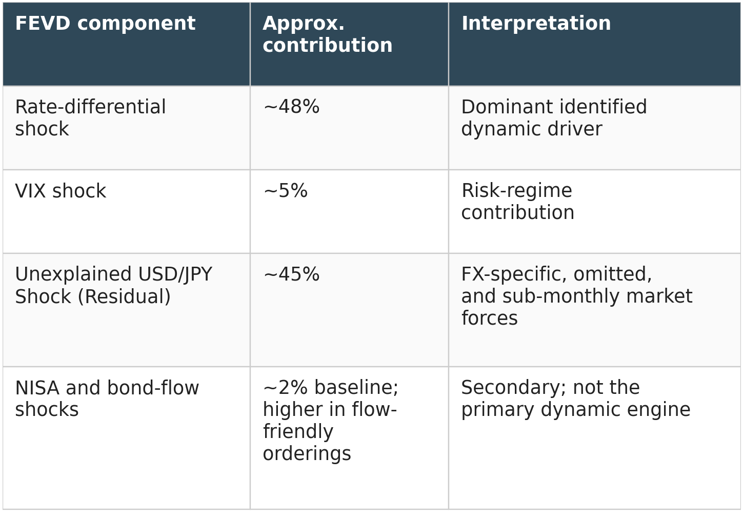
The VAR result supports the same hierarchy as the monthly attribution model: rate differentials are the cleanest identified driver, while public flow proxies are best framed as light structural pressures rather than the main monthly causal engine. The Cholesky ordering is an identification assumption, not proof of causality, so the article treats the result as causal-style attribution under explicit assumptions.
Part IV - Final Horizon Response: Local Projections
Local projections provide a second dynamic check. Instead of imposing one VAR impulse-response path, they estimate the cumulative USD/JPY response at multiple horizons after a standardized shock. This is useful because exchange-rate responses might decay or reverse over time.
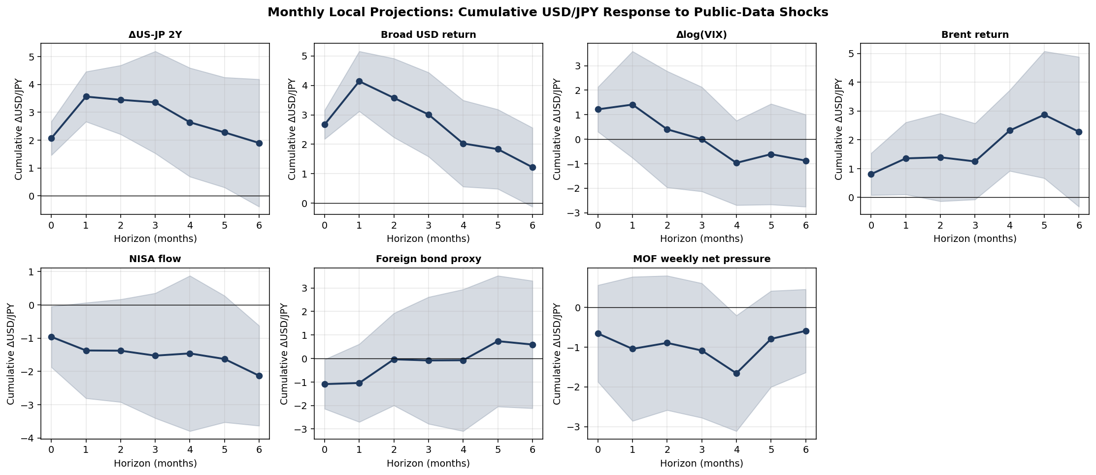
Figure 5. Local projections. Rate and broad-dollar shocks produce the most stable, correctly signed responses. Flow proxies are weaker and often wrong-signed.
The local-projection layer reinforces the final model hierarchy. The strongest responses are produced by rate-differential and broad-dollar shocks. Flow shocks responses are less important in magnitude.
Part V - Probability Methodology: Public-Data Scenario Calibration
The scenario probabilities are calibrated from public market and official information, then constrained by the empirical hierarchy of the model. Because the attribution work identifies the U.S.-Japan rate differential as the dominant USD/JPY driver, the U.S. macro/rates axis remains the first probability axis. Japan policy and energy risk are then estimated conditionally on that U.S. state. Flow pressure and intervention are treated as amplifiers and path constraints rather than separate first-order probability axes.
The probabilities should therefore be read as evidence-weighted scenario probabilities, not as direct regression outputs or risk-neutral options probabilities. They are reproducible because the inputs can be updated from public sources at each publication date.
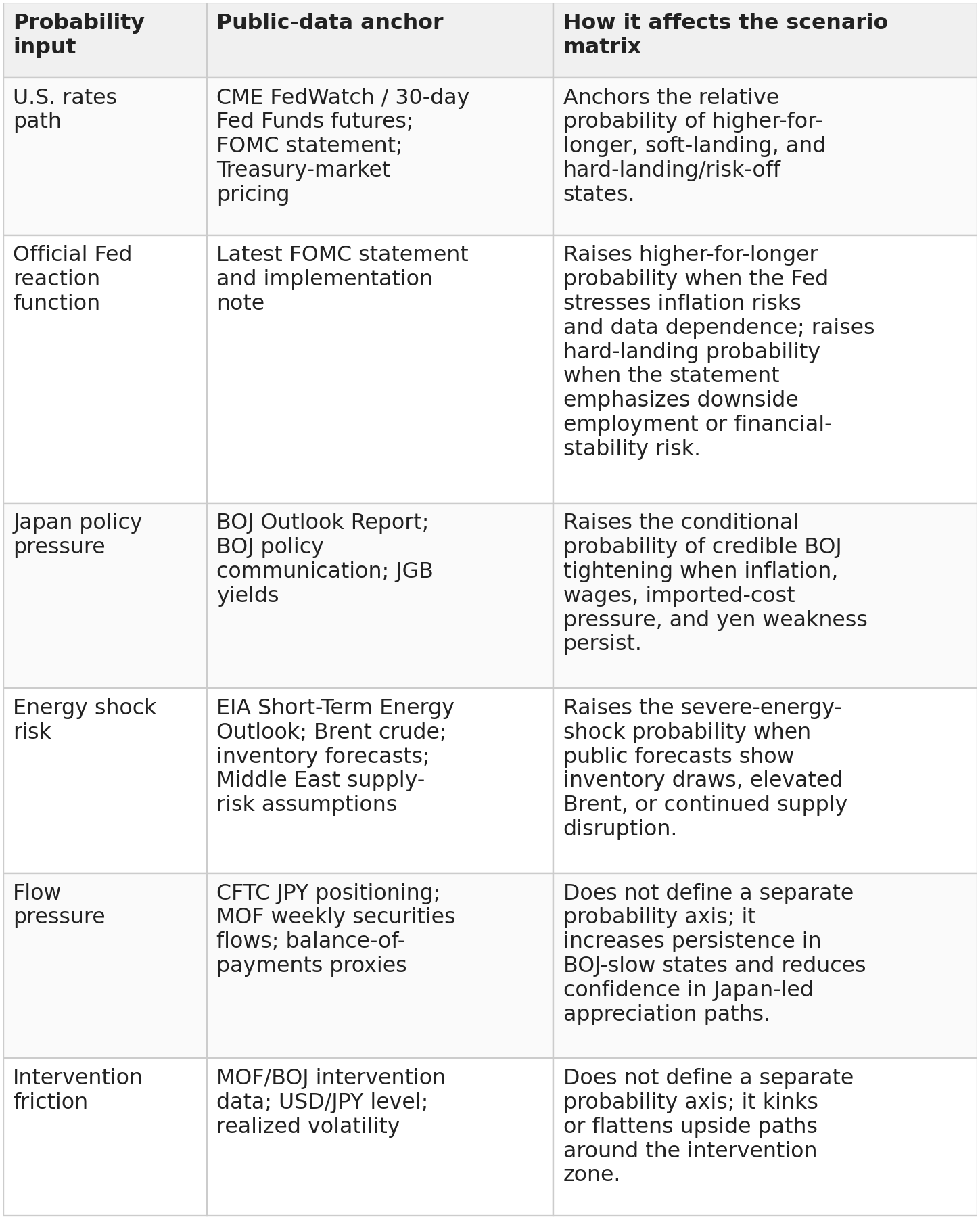
Public-source calibration rule
Joint probabilities are calculated as: P(U.S. macro/rates state) x P(Japan policy state | U.S. state) x P(Energy state | U.S. state). The U.S. state probabilities are anchored first to market-implied policy-rate probabilities and then adjusted by a macro/risk score. Conditional Japan-policy and energy probabilities are anchored to official BOJ and EIA information. The calculation is intentionally simple enough to be audited and updated.
Operationally, calibration is done in four auditable steps:
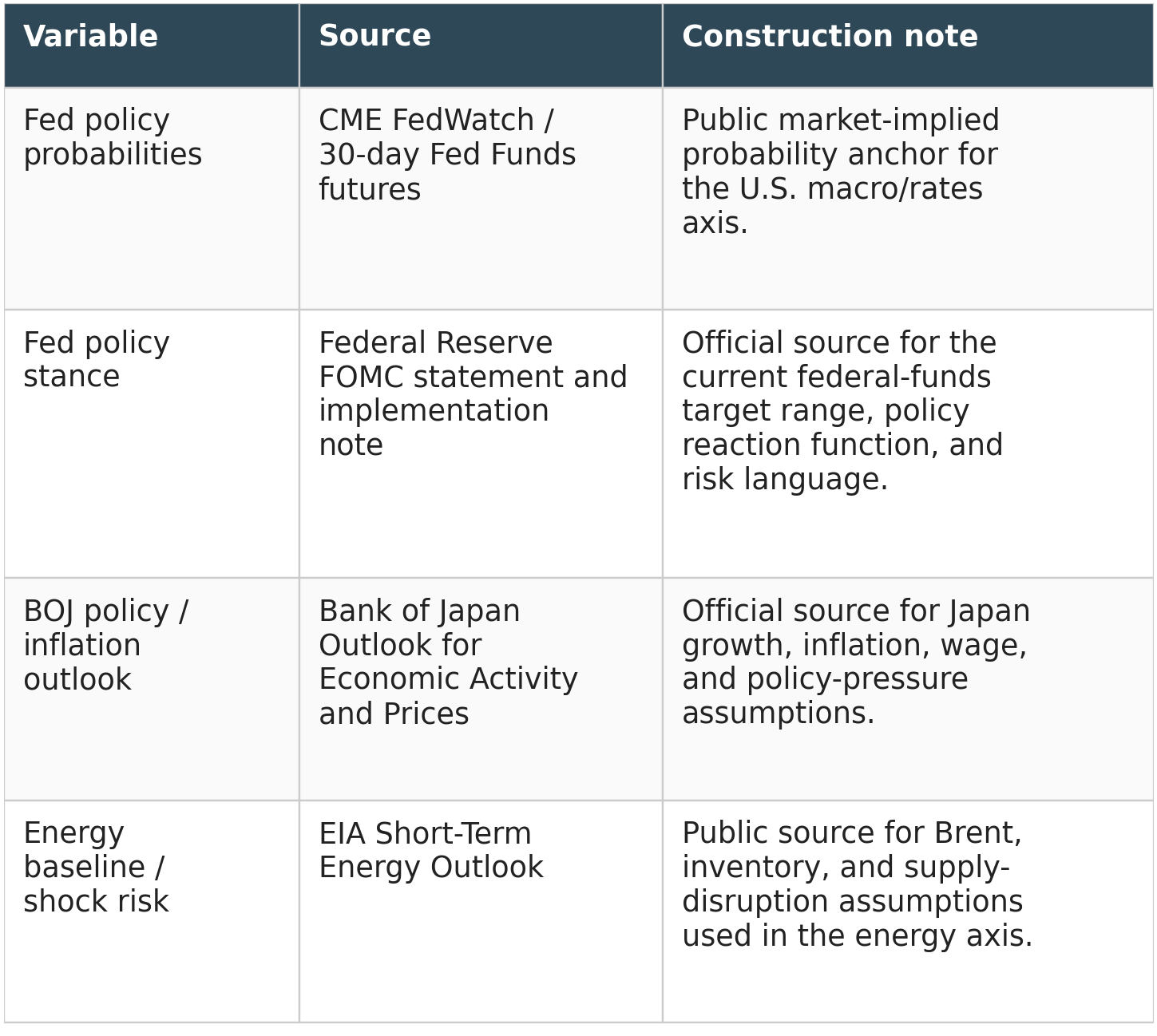
1. Read public inputs at the publication date: FedWatch/Fed funds futures for the policy-rate path, the latest FOMC statement, U.S.-Japan yield spreads, VIX/credit-risk indicators, the BOJ Outlook Report, JGB pricing, Brent crude, and the EIA Short-Term Energy Outlook.
2. Normalize each signal into a simple 0-1 evidence score. For example, a high probability of no or limited Fed cuts increases the higher-for-longer score; a large expected easing path plus wider credit stress increases the hard-landing/carry-unwind score; BOJ inflation and yen-stress evidence increase the credible-tightening score; and EIA inventory draws plus Brent prices above the baseline increase the energy-shock score.
3. Convert the public anchors into a blended probability allocation. The higher-for-longer bucket is anchored to Fed funds futures/FedWatch-style rate pricing and then adjusted down because it is broader than a Fed-unchanged event. The hard-landing bucket is anchored to public recession-risk evidence and adjusted only slightly for volatility/carry-unwind risk. The soft-landing bucket is the residual probability after those two buckets are set.
4. Estimate Japan-policy and energy probabilities conditionally on the U.S. state, then multiply: P(final scenario) = P(U.S. state) x P(Japan state | U.S. state) x P(energy state | U.S. state). The final outlook table is therefore an auditable transformation of public evidence rather than a direct regression forecast.
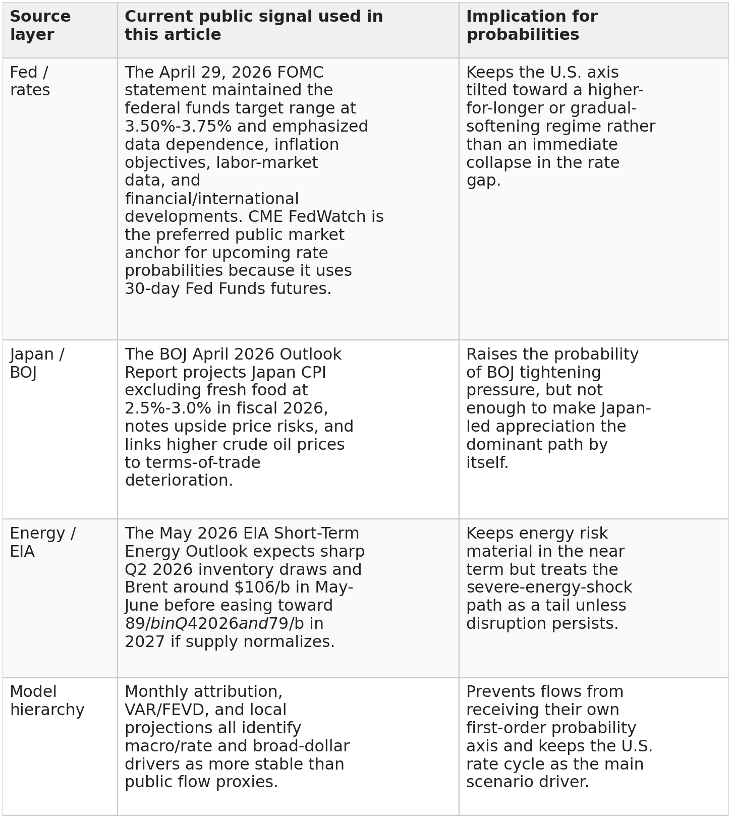
Current public-data calibration
Using the public signals above, the current calibration adopts a blended U.S. macro/rates allocation: 55% higher for longer, 27% soft landing, and 18% hard landing + VIX. The blend deliberately does not copy any single public-source number mechanically. Instead, each public source is treated as an anchor for a narrower observable event, and the article adjusts that anchor depending on whether the USD/JPY scenario bucket is broader or narrower than the source event.
The higher-for-longer bucket starts from Fed funds futures / CME FedWatch-style pricing of limited easing or unchanged rates. That public rate-pricing anchor is adjusted down because “Fed unchanged” is not identical to a sustained USD/JPY upside regime. USD/JPY can still move sideways or lower if the broad dollar weakens, JGB yields rise, BOJ credibility improves, or intervention pressure increases. The scenario therefore remains the largest U.S. state, but its probability is discounted from the raw unchanged-rate anchor.
The hard-landing + VIX bucket is anchored to public recession-risk evidence, especially yield-curve/recession-probability models and observable volatility or credit-stress indicators. It is rounded only slightly upward because a USD/JPY carry unwind can occur through a volatility shock even without a formal recession. The adjustment is kept small because benign credit spreads and non-crisis financial-stability indicators argue against making the hard-landing bucket dominant.
The soft-landing bucket is the residual probability after the higher-for-longer and hard-landing states are assigned. It is lower than higher for longer because Fed communication and market pricing still support restrictive policy. It is higher than the hard-landing bucket because public credit and recession-risk evidence do not point to a dominant recession scenario.
This produces the following blended U.S. probabilities: P(higher for longer) = 55%, P(soft landing) = 27%, and P(hard landing + VIX) = 18%. The purpose is to make the adjustment direction auditable: rate-market evidence is discounted when it is narrower than the USD/JPY regime, recession evidence is preserved almost one-for-one, and the soft-landing probability absorbs the remaining non-crisis probability mass.
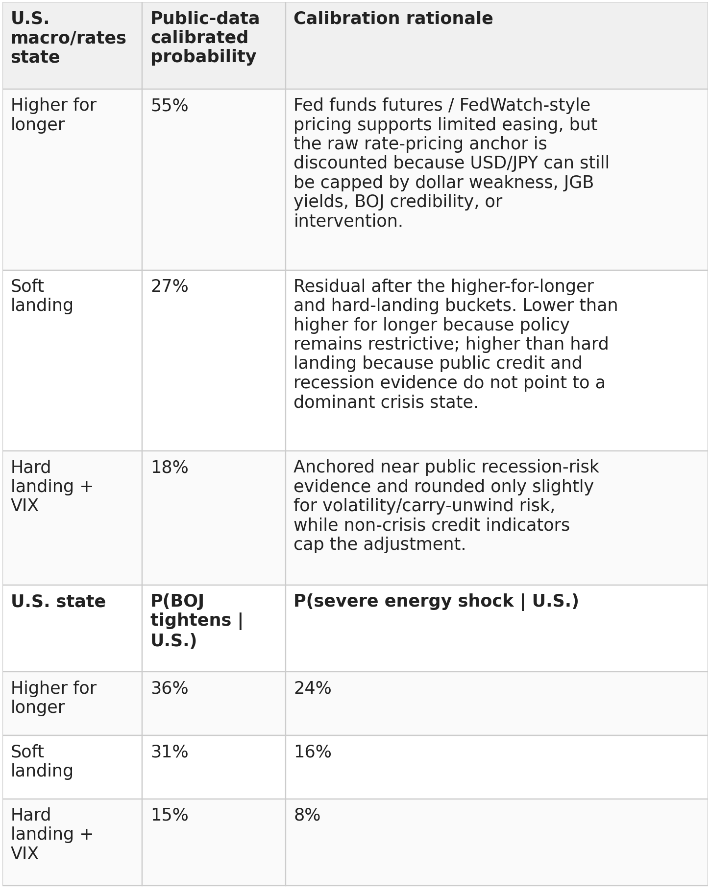
The calibration is designed to be updated. At each refresh, the FedWatch probability table, the latest FOMC statement, BOJ Outlook Report, EIA STEO, Brent crude, VIX, and yield-spread data should be re-read. The scenario probabilities should then be recalculated from the same rules rather than manually overwritten.
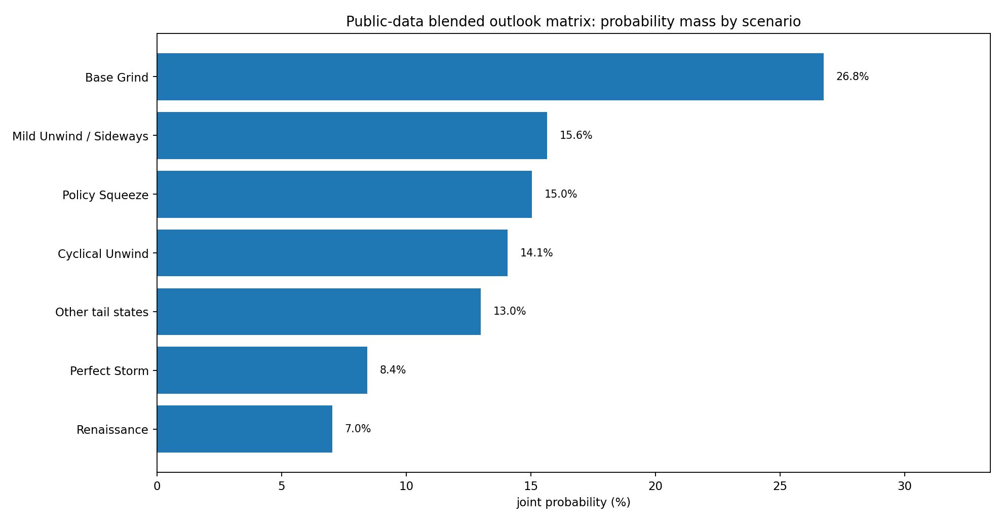
Figure 8. Public-data calibrated outlook matrix. The chart shows the updated probability mass after translating public rates, BOJ, energy, and risk evidence into the joint scenario matrix.
Part VI - How the Model Maps Into Forecast Paths
The forecast paths remain heuristic scenario trajectories rather than direct regression point forecasts. What changes is the source of the probability weights: the path logic still comes from the empirical model hierarchy, while the probability mass comes from public market and official information.
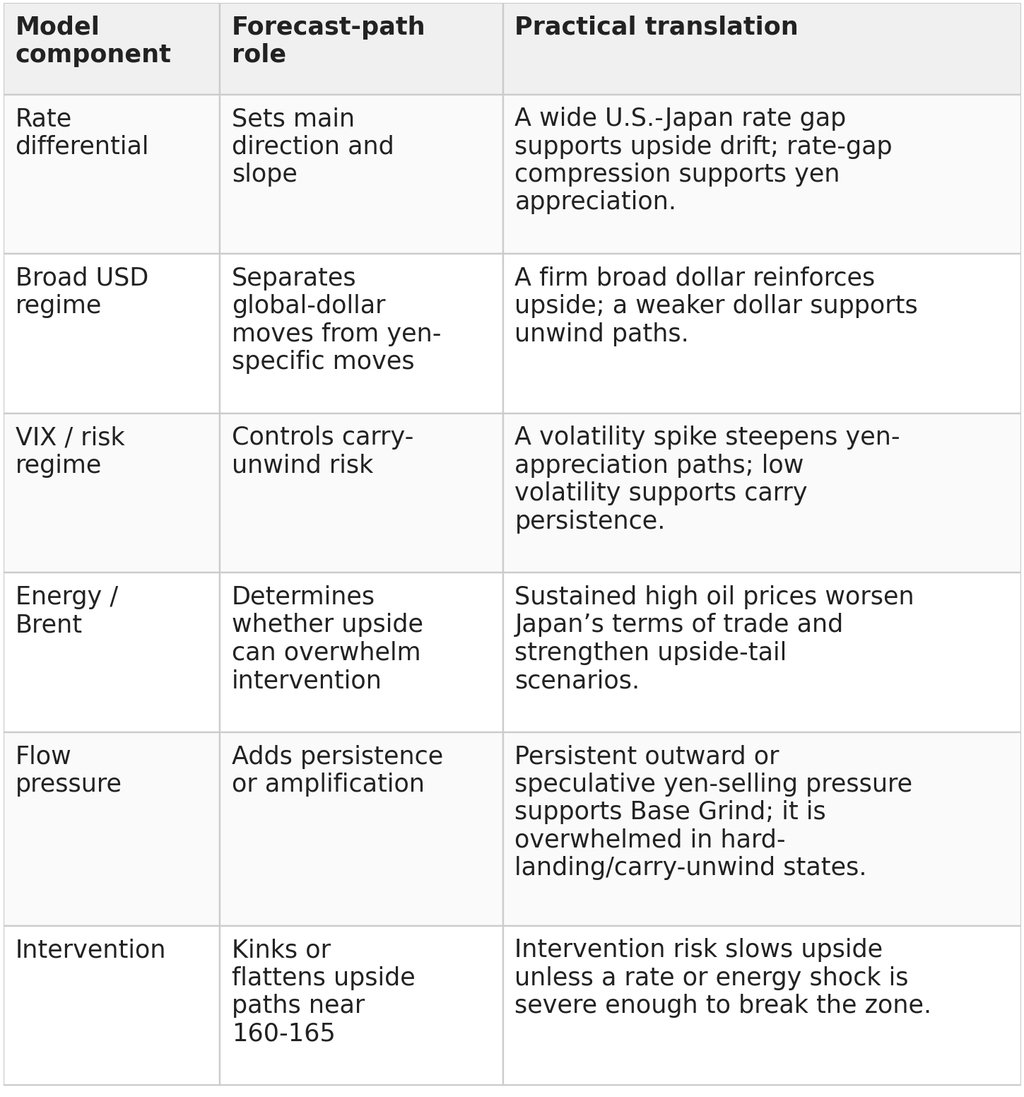
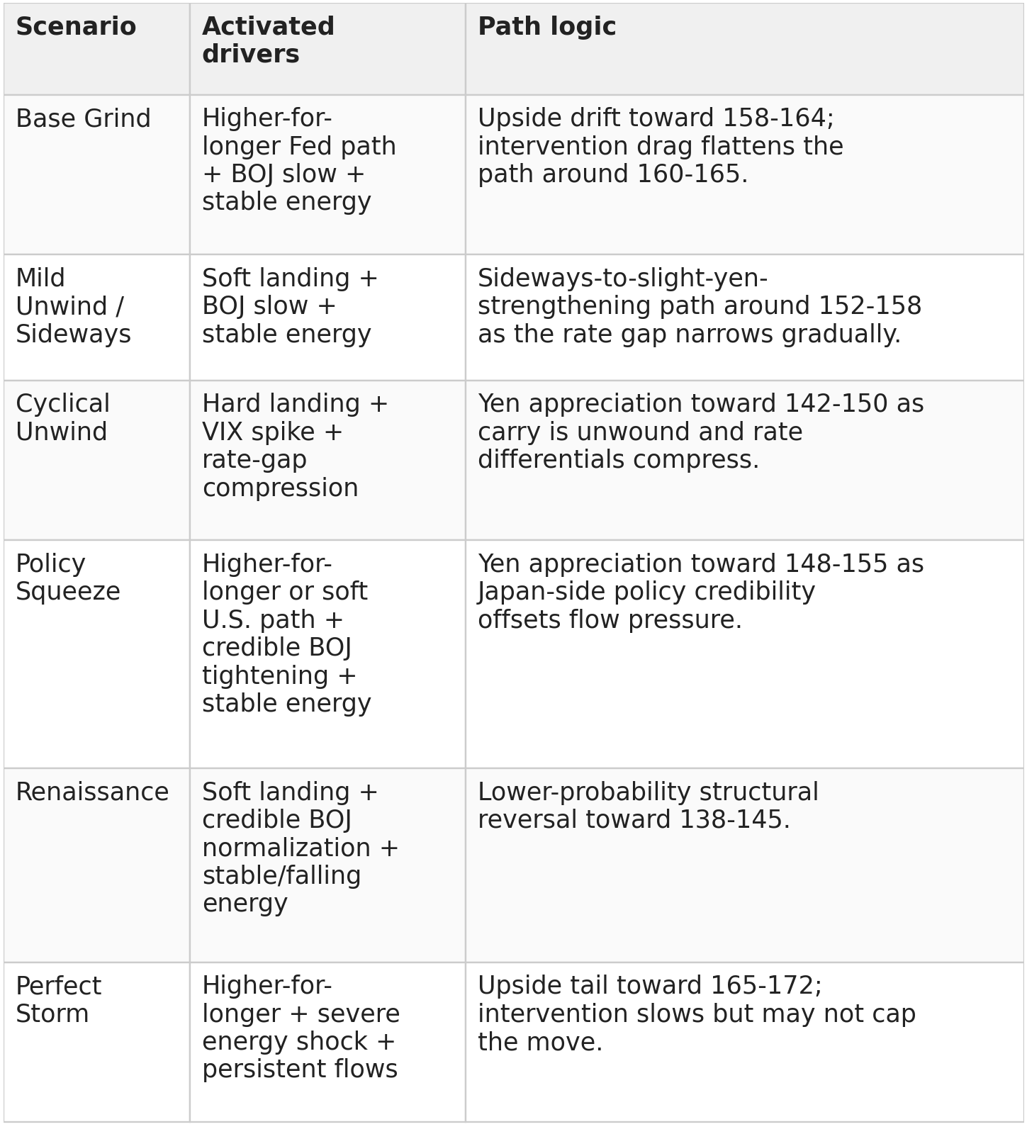
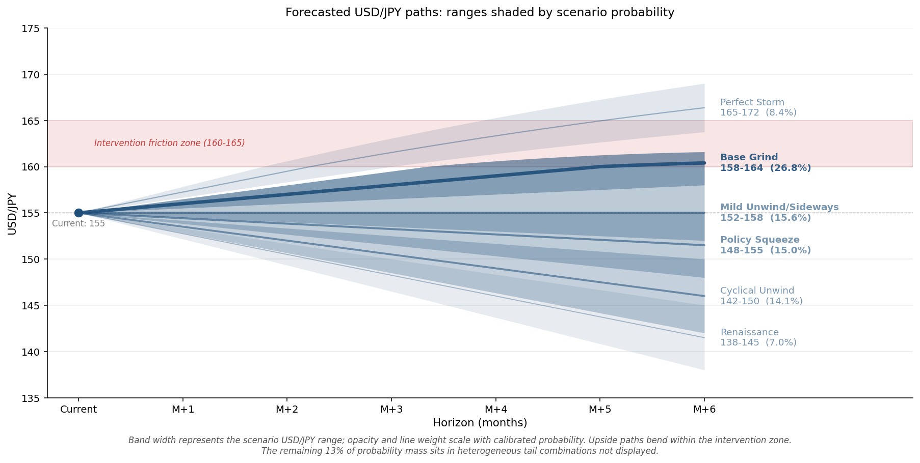
Figure 9. Forecasted USD/JPY paths. Path shapes are still heuristic and model-constrained, but line thickness and likelihood shading now reflect the public-data calibrated scenario probabilities.
Part VII - Public-Data Calibrated Outlook Matrix
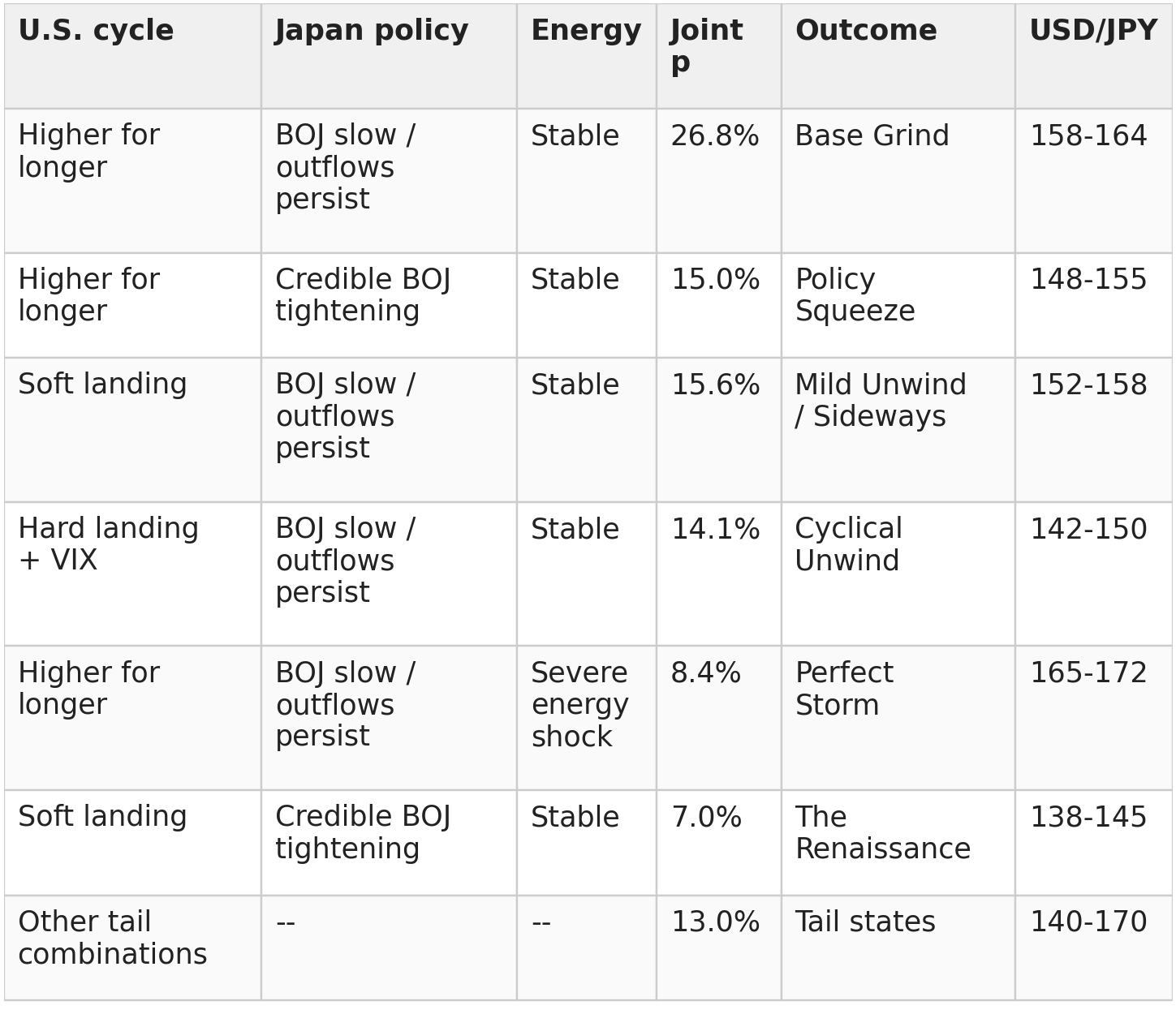
The outlook matrix below uses the updated blended public-data calibration. Compared with the previous internally assigned matrix, the highest-probability path is Base Grind, but Policy Squeeze and Mild Unwind / Sideways remain material because the calibration discounts the raw Fed-unchanged anchor and reserves meaningful probability for gradual rate-gap compression or BOJ credibility.
Matrix interpretation
The largest single scenario is Base Grind at roughly 26.8%, but it should not be read as certainty. The next-largest paths are Policy Squeeze and Mild Unwind / Sideways, both around the mid-teens. This is intentional: public policy and energy data still support yen vulnerability, but the blended calibration does not equate an unchanged Fed path with guaranteed USD/JPY upside.
The most important yen-appreciation path is a U.S.-led cyclical unwind: rate-gap compression and volatility-driven carry reduction. The most important upside tail is still a higher-for-longer U.S. rate regime combined with a severe energy shock and persistent flow pressure. BOJ tightening matters, but the model and public calibration suggest that Japan policy alone is less likely to dominate USD/JPY unless it coincides with U.S. rate-gap compression or lower energy pressure.
What would force recalibration?
· CME FedWatch or Fed Funds futures reprice toward faster rate cuts or renewed hikes.
· The U.S.-Japan 2-year spread compresses by 40 basis points or more over a quarter.
· The BOJ signals faster rate normalization or accelerates JGB-purchase tapering.
· The EIA/IEA baseline changes materially, Brent remains above the current baseline, or the Strait of Hormuz / Middle East risk premium persists longer than expected.
· Confirmed intervention data show repeated operations large enough to alter expectations rather than simply smooth volatility.
· CFTC Leveraged Money positioning develops a sustained lead on USD/JPY at higher frequency.
Public sources used for the probability calibration: CME FedWatch / 30-day Fed Funds futures; Federal Reserve FOMC statement and implementation note of April 29, 2026; Bank of Japan Outlook for Economic Activity and Prices, April 2026; U.S. Energy Information Administration Short-Term Energy Outlook, May 2026; FRED / Treasury yield data; CFTC Commitment of Traders; MOF weekly securities-flow data.
Conclusion
The public-data evidence points to a clearer and more defensible interpretation of USD/JPY than a pure structural-flow narrative. Public flows matter, but they are not the main monthly engine. The engine is the macro price of money: U.S.-Japan rate differentials, the broad dollar regime, risk appetite, and energy-sensitive terms of trade. Flow pressure reinforces those regimes, but it does not replace them.
The Ministry of Finance can slow disorderly moves and defend psychologically important levels, but intervention is an endogenous friction rather than the underlying driver. That is why the forecast paths show explicit intervention effects: upside paths flatten around the 160-165 zone unless a severe rate or energy shock overwhelms the defense. In the base case, the yen remains vulnerable but capped by intervention risk; in the main appreciation scenario, the yen strengthens because the U.S. cycle turns, not because Japanese flow pressure suddenly disappears.
The result is an attribution framework that is both empirical and transparent. Monthly attribution, VAR/FEVD, and local projections all point to the same hierarchy. The conditional probability matrix then uses that hierarchy to organize uncertainty. The article’s strongest claim is therefore not that a model can forecast USD/JPY precisely, but that the right first axis for any USD/JPY outlook is the U.S. macro/rates cycle, with flows and intervention treated as amplifiers and constraints.
Appendix A - Data Sourcing and Proxy Construction
Appendix B - Econometric Methodology
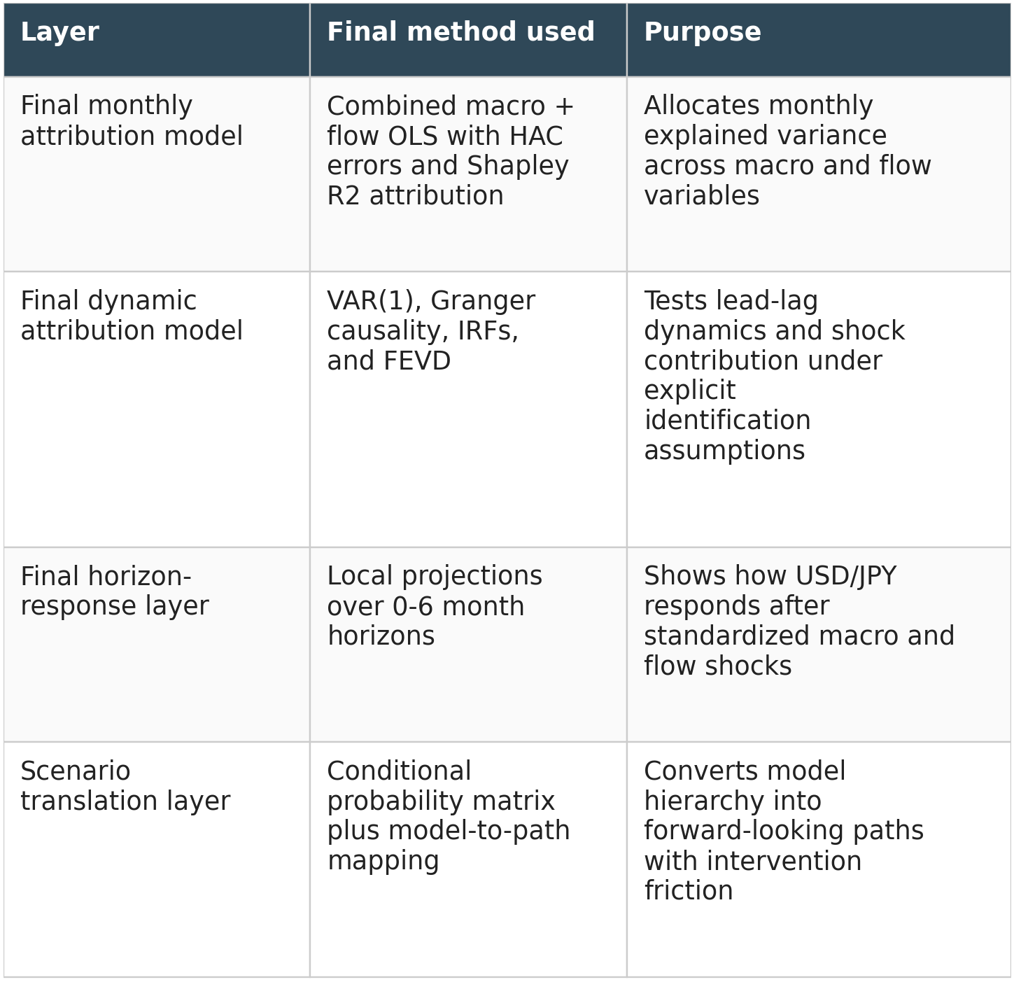
Monthly OLS is estimated with HAC robust standard errors because FX returns can exhibit heteroskedasticity and autocorrelation. Shapley decomposition is used to allocate explained R2 under multicollinearity. The VAR(1) layer estimates dynamic attribution through Granger tests, impulse-response functions, and forecast-error variance decomposition. Local projections estimate horizon-specific cumulative responses to standardized shocks.
The central regression can be summarized as: Delta USDJPY_t = alpha + beta_macro * Macro_t + beta_flow * Flow_t + error_t. Shapley attribution evaluates the marginal contribution of each variable across all possible model subsets, preventing highly correlated predictors from receiving attribution solely because of ordering in the regression specification.
The dynamic layer uses a parsimonious VAR because the sample is short. The baseline ordering places rate-differential and VIX shocks before USD/JPY and places public flow proxies after USD/JPY. This is economically defensible because monthly Japanese retail or bond-flow proxies are unlikely to be more exogenous than the Fed/BOJ rate environment. Nevertheless, the result is described as causal-style attribution under assumptions, not causal proof.
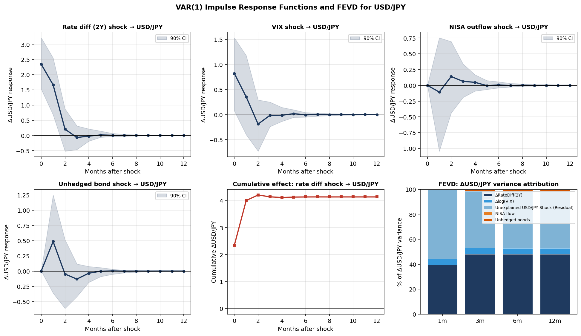
Appendix Figure B1. VAR impulse-response functions and FEVD details. Rate shocks have the clearest immediate effect; flow shocks have weaker and less stable responses.
Appendix C - Methodology Comparisons and Robustness Checks
The main body reports only the final models. This appendix documents the main specification comparisons and robustness checks that led to the final framework.
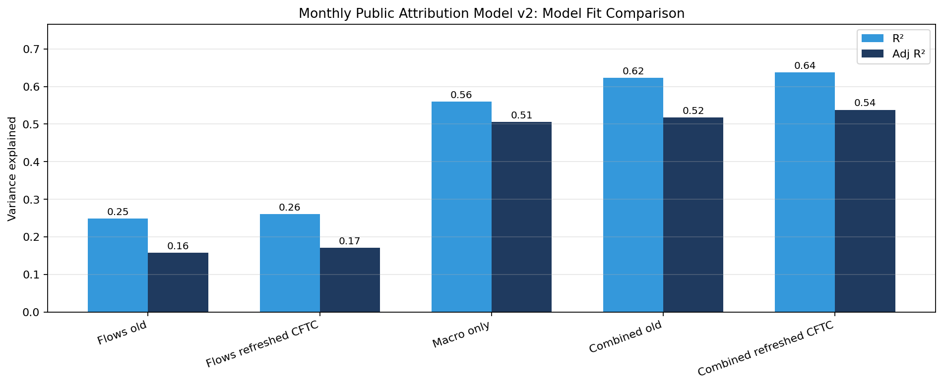
Appendix Figure C1. Public attribution model comparison. Macro variables dominate the association layer; flows add context but are not the primary model. This comparison is diagnostic and is not part of the main body’s final model narrative.
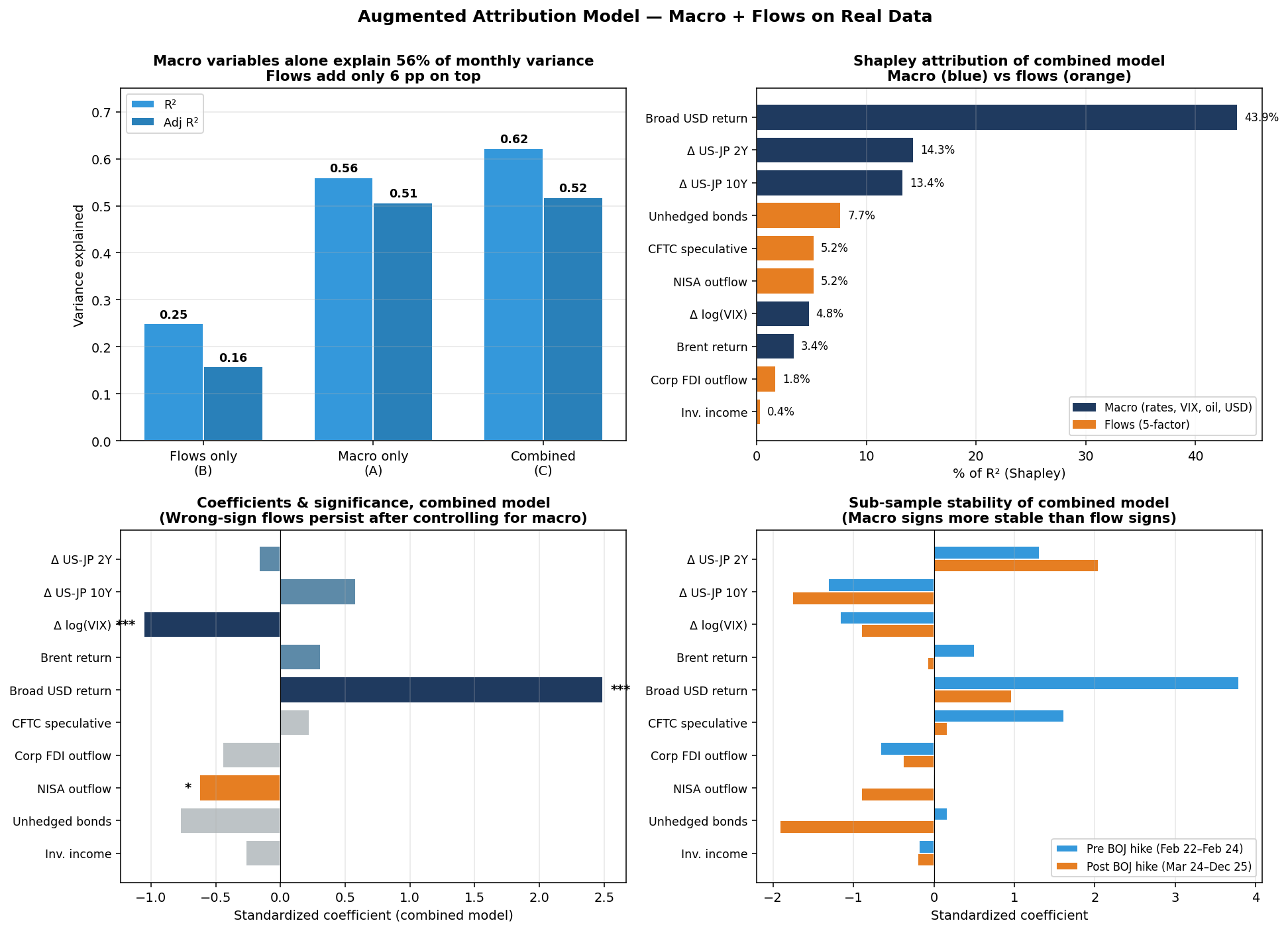
Appendix Figure C2. Augmented model diagnostics. The combined model improves fit, but flow signs remain unstable relative to macro variables.
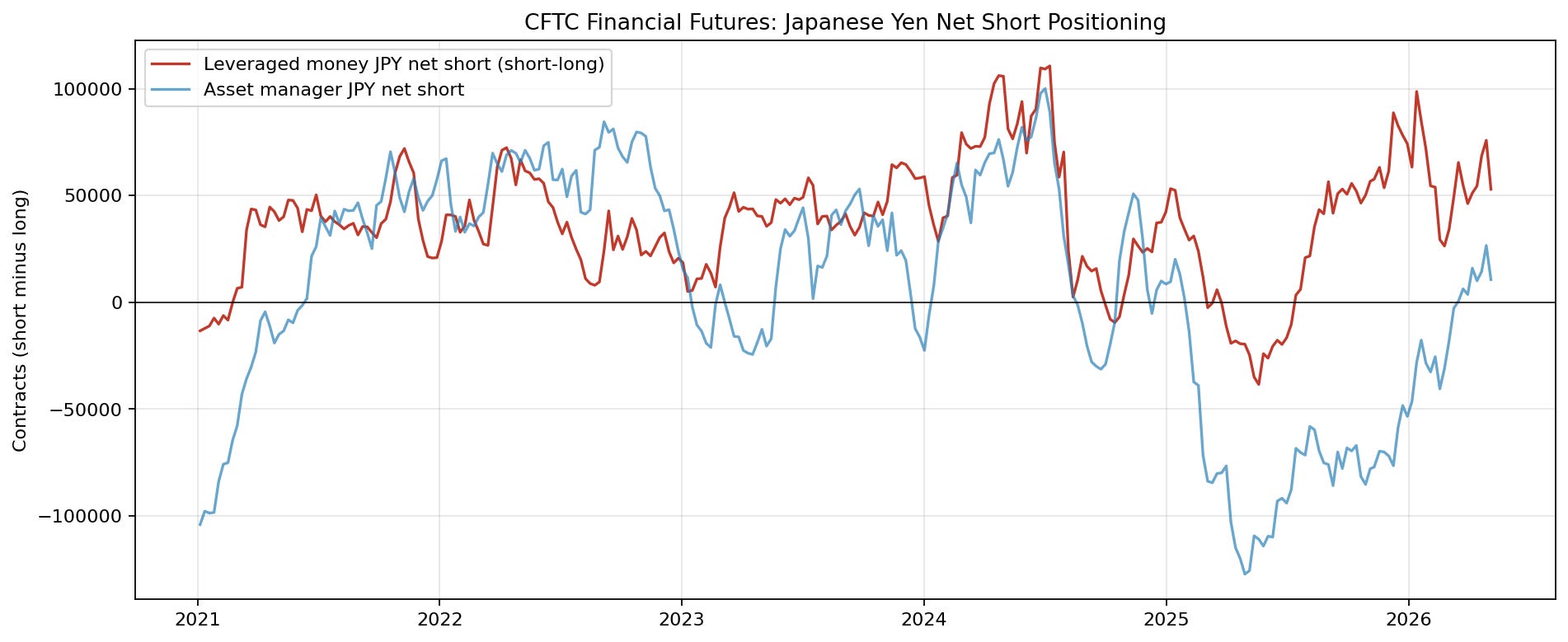
Appendix Figure C3. CFTC financial futures positioning. Leveraged Money is the relevant CFTC sub-category for near-term speculative positioning.
Acknowledgement on AI Assistance
This article was produced with assistance from three large language models: Claude (Anthropic), Grok, ChatGPT (OpenAI), and Google Gemini. AI assistance was used for code generation, statistical implementation, literature scoping, drafting and editing of prose, and iterative methodology critique. The analytical design, choice of data sources, interpretation of results, scenario construction, and final claims are the author’s own. All errors of fact, judgment, or interpretation remain the author’s responsibility.
Disclaimer: This research is for informational purposes only and should not be interpreted as investment advice, a recommendation, or an offer to buy or sell any financial instrument.